Thi Thanh Nga Nguyen![]()
© 2023 IIETA. This article is published by IIETA and is licensed under the CC BY 4.0 license (http://creativecommons.org/licenses/by/4.0/).
OPEN ACCESS
This study introduces a novel computational approach for optimizing the design of cam knife-edge followers by utilizing potential energy analysis. In this methodology, cam parameters are succinctly represented using curvilinear coordinate systems, and the objective function is derived from the potential energy. To stabilize the position between two points, a stabilization function is incorporated. The cam curve is discretized through finite element analysis, and the resulting nonlinear equation is solved using the Newton-Raphson method. Additionally, the optimal design of the cam knife-edge follower considers cam size, which is associated with the base circle radius and pressure angle. Results demonstrate that the proposed method offers greater flexibility in evaluating and optimizing the design parameters of cam knife-edge followers compared to existing approaches. This study not only provides new insights into the optimization of cam knife-edge followers but also has potential applications in other related fields.
cam curve, cam knife-edge follower, curvilinear coordinate, potential energy, finite element discretization, newton-Raphson method, pressure angle
Cam-follower mechanisms, featuring flexible motions generated by cam curves, have been widely employed in various applications, such as engines [1-6], fuel pumps [6], and indexing cam mechanisms [7, 8]. In cam system computations, accurately describing the follower motion is crucial, as it influences the cam motion characteristics, including kinematics and dynamics. Several transfer functions have been employed for modeling follower motions, including trigonometric functions [9-12], polynomials [13-15], and spline functions [16-19].
Concerning the kinematics and dynamics of cam follower motion, Zhou et al. [1] investigated the effects of design methods on the profiles of intermediate cams in variable valve lift systems. By employing a kinematic model, cam profiles were obtained, and the kinematic behavior of cam systems was determined. Sun et al. [20] proposed an optimization approach for cam mechanisms' motion curves, aiming to achieve the lowest maximum acceleration. Optimal kinematic characteristics of cam mechanisms were examined using NURBS for the follower function [18]. Further research focused on enhancing the accuracy of kinematics and dynamics for conjugate cam mechanisms, thereby reducing system vibration [21, 22]. A polynomial fitting-based design for electronic cams [23].
Alaci et al. [24] proposed a cam curvature for cam knife-edge followers, which have been used in engines and fuel pumps, and simulated using finite element analysis on CATIA software [6]. In cam curve design, John et al. [25] and Myszka [26] introduced graphical and analytical methods for determining cam curves. However, these studies did not address cam curve optimization and did not consider design parameters for cam knife-edge followers. To date, there has been a lack of research on the optimal design of cam knife-edge mechanisms. Notably, the computation of cam curves constitutes an essential step in the design of cam knife-edge follower mechanisms, as the base circle radius affects the pressure angle and cam size. The pressure angle, in turn, influences the transmission ability between the cam and the follower. Consequently, this study aims to develop a novel method for optimizing the cam curve of cam knife-edge followers, which considers not only the cam mechanism size but also the pressure angle. The potential energy is employed as the objective function, and the finite element method is utilized for computing the problem. The Newton-Raphson method is subsequently implemented to solve the proposed problem.
The remainder of this study is organized as follows: Section 2 presents the formulation of the optimization problem. Section 3 introduces the finite element method for computing the cam curve. Section 4 describes the Newton-Raphson algorithm for problem-solving. Section 5 discusses the results, and finally, conclusions are provided in Section 6.
This section presents the procedure in order to build the objective function for designing the cam curve of the cam knife-edge follower. The cam curve is achieved from the “deformation” of the initial curve. The description of the cam curve is shown in the section below.
2.1 Description for cam knife-edge follower
The description of cam knife-edge follower is shown in Figure 1. The initial cam curve, denoted by Co(x), is chosen as a circle. The circle is defined as the base circle of the cam knife-edge follower. The current curve (cam curve), denoted by C(x), is obtained from the “deformation” of the initial curve. The cam curve is described by the curvilinear coordinate systems. The tangent vectors on the initial and current cam curves are respectively denoted by A1 and a1, d and n are described for the follower motion direction and normal vector of cam curve, respectively. The transfer function of the follower, denoted by y, presents the lift of the follower movement.
Figure 1. Geometry description of cam knife-edge follower
In order to compute the cam curve, the transfer function must be given. In general, the given transfer function, denoted by yo, is a function that depends on the angle of cam shaft. It can be written as:
$y_0=f(\alpha)$, (1)
where, $\alpha$ is angle of cam shaft. It can be calculated from Figure 1.
$\alpha=\operatorname{acos}\left(\mathbf{d} \cdot \mathbf{x}_1\right)$. (2)
The desired cam curve can be described by using the curvilinear coordinate $\xi$ as shown in Eq. (3).
$\mathbf{x}=\mathbf{x}(\xi)$. (3)
The tangent vector a1 and a1 of the co-variant and contra-variant to coordinate $\xi$ at x on the current curve C(x) are:
$\mathbf{a}_1=\frac{\partial \mathbf{x}}{\partial(\xi)}$, (4)
$\mathbf{a}^1=\mathbf{a}^{11} \mathbf{a}_{\mathbf{1}}$. (5)
The contra-variant basis and the co-variant basis at x of the current cam curve, denoted by a11 and a11, can be computed as:
$a_{11}=\mathbf{a}_1 \cdot \mathbf{a}_1$, (6)
$a^{11}=\left[a_{11}\right]^{-1}$. (7)
The geometry parameters on the initial curve are likewise determined with the current curve.
The current transfer function is computed from Figure 1.
$y=\mathbf{x} \cdot \mathbf{d}-r_o$, (8)
in which, ro is base circle radius. The follower motion direction d can be calculated by:
$\mathbf{d}=\frac{\mathbf{x}}{\|\mathbf{x}\|}$. (9)
The normal vector n is determined as:
$\mathbf{n}=\frac{\mathbf{a}_{\mathbf{1}}}{\left\|\mathbf{a}_{\mathbf{1}}\right\|}$. (10)
2.2 Objective function
As discussion above, the initial cam curve is deformed to create the cam curve. In order to obtain the desired cam curve, the difference between the given transfer function yo and the current transfer function y must be equal to zero (y-yo=0). To impose the constraint of the transfer function, the potential energy, denoted by $\Pi_p$, is used to express the objective function as follows:
$\Pi_p=\frac{k}{2} \int_\alpha\left(y-y_o\right)^2 \mathrm{~d} \alpha$, (11)
where, k is constant parameter.
For only the constraint of the transfer function during the deformation, this is not enough to stabilize the position between two points, thus the constraint of stabilization is added to the solution. Using the numerical stabilization [27], the stabilized constraint, denoted by $\Pi_s$, can be expressed as:
$\Pi_s=\frac{\mu}{2} \int_\alpha\left(A^{11} a_{11}-2 \ln \frac{\left\|\mathbf{a}_1\right\|}{\left\|\mathbf{A}_1\right\|}\right)^2 \mathrm{~d} \alpha$, (12)
in which, $\mu$ is stabilized parameter. The other parameters, i.e., A11, a11, a1, A1 are calculated in the previous section.
From Eq. (11) and Eq. (12), the cam curve is obtained by minimizing the following equation:
$\begin{gathered}\min \Pi=\Pi_p+\Pi_s =\frac{k}{2} \int_\alpha\left(y-y_o\right)^2 \mathrm{~d} \alpha+ \frac{\mu}{2} \int_\alpha\left(A^{11} a_{11}-2 \ln \frac{\left\|\boldsymbol{a}_1\right\|}{\left\|\boldsymbol{A}_1\right\|}\right)^2 \mathrm{~d} \alpha\end{gathered}$ (13)
2.3 Variation of the design function
The variation of design function needs to be computed for minimizing Eq. (13). Taking the variation of the potential energy as shown in Eq. (11) is:
$\delta \Pi_p=k \int_\alpha\left(y-y_o\right)\left(\delta y-\delta y_o\right) \mathrm{d} \alpha$, (14)
where, $\delta y_o$ and $\delta y$ are calculated from Eq. (1) and Eq. (8). Computing $\delta y_o$ and $\delta y$, and then substituting into Eq. (14), the variation of the potential energy leads to:
$\delta \Pi_p=k \int_\alpha\left(y-y_o\right) \mathbf{b} . \delta \mathbf{x} \mathrm{d} \alpha$, (15)
in which, the vector b is set by:
$\mathbf{b}=\mathbf{d}+\mathbf{B r}$. (16)
In Eq. (16), the second-order tensor B and the vector r are computed as:
$\begin{gathered}\mathbf{B}=\frac{1}{\|\mathbf{x}\|}(\mathbf{I}-\mathbf{d} \otimes \mathbf{d}), \mathbf{r}=\mathbf{x}+c_1 \boldsymbol{x}_{\mathbf{1}}\end{gathered}$ (17)
Here, I is the second-order identity tensor and $\mathrm{c}_1=\frac{\partial y_o}{\partial \alpha} \frac{1}{\sqrt{1-\cos \alpha^2}}$.
Likewise, the variation of the stabilization constraint is computed as:
$\delta \Pi_s=\mu \int_\alpha\left(A^{11}-a_{11}\right) \boldsymbol{a}_1 . \boldsymbol{\delta} \boldsymbol{a}_1 \mathrm{~d} \alpha$. (18)
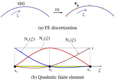
This section presents the finite element (FE) method for solving Eq. (13). The discretized form is presented by finite element discretization of the curve. The node is denoted by Xe.
3.1 Finite element discretization
For cam curve, the quadratic finite element in 1D is used for computation. The FE discretization of cam curve is shown in Figure 2 (a). The shape function of the quadratic finite element is presented in Figure 2 (b). The shape function can be expressed as $\mathrm{N}_i=\mathrm{N}_i(\xi)$.
Figure 2. FE discretization and quadratic finite element of cam curve
In each element, the geometry is approximated by the nodal interpolations:
$\mathbf{x}=\sum_{e=1}^n \mathbf{N} \mathbf{x}_{\mathbf{e}}$, (19)
where, $\mathbf{N}=\mathbf{N}(\xi)$ and n is the number of nodes, respectively. Eq. (19) and Eq. (4) can be written by shorthand notation:
$\mathbf{x}=\mathbf{N} \mathbf{x}_{\mathrm{e}}$, (20)
$\mathbf{a}_1=\mathbf{N}_{, \xi} \mathbf{x}_{\mathrm{e}}$, (21)
with $\mathbf{N}_{, \xi}=\mathbf{\partial N} / \partial \xi$. The variation of x and a1 is written as:
$\delta \mathbf{x}=\mathbf{N} \delta \mathbf{x}_{\mathbf{e}}$, (22)
$\delta \mathbf{a}_{\mathbf{1}}=\mathbf{N}_{, \xi} \delta \mathbf{x}_{\mathbf{e}}$, (23)
3.2 Discretized form equation
By substituting the finite element discretization in Eq. (22) and Eq. (23) into Eq. (15), the variations of the potential energy in discretized form $\delta \Pi_s^e$ can be rewritten as:
$\delta \Pi_p^e=\delta \mathbf{x}_{\mathbf{e}}^{\mathbf{T}} \int_{\alpha_e} \mathbf{N}^{\mathbf{T}} k\left(y-y_o\right) \mathbf{b} \cdot \mathrm{d} \alpha_e$, (24)
Likewise, substituting the finite element discretization in Eq. (22) and Eq. (23) into Eq. (18), the variation of stabilized constraint equation in the discretized form $\delta \Pi_s^e$ is:
$\delta \Pi_s^e=\delta \mathbf{x}_{\mathbf{e}}^{\mathbf{T}} \int_{\alpha_e} \mathbf{N}_{, \zeta}^{\mathbf{T}} \mu\left(A^{11}-a_{11}\right) \boldsymbol{a}_1 \cdot \mathrm{d} \alpha_e$. (25)
The cam curve is obtained when the variation of both the potential energy and the stabilized constraint equation in discretized form is set to zero for all variation $\delta \mathbf{x}_e$. From Eq. (24) and Eq. (25), the total discretized from equation can be written as:
$\begin{gathered}\delta \Pi^e=\delta \Pi_p^e+\delta \Pi_s^e =\delta \mathbf{x}_{\mathbf{e}}^{\mathrm{T}}\left(\int_{\alpha_e} \mathbf{N}^{\mathrm{T}} k\left(y-y_o\right) \mathbf{b} \cdot \mathrm{d} \alpha_e+\right. \left.\int_{\alpha_e} \mathbf{N}_{, \xi}^{\mathrm{T}} \mu\left(A^{11}-a_{11}\right) \boldsymbol{a}_1 \cdot \mathrm{d} \alpha_e\right)=0 \forall \delta \mathbf{x}_e\end{gathered}$ (26)
3.3 Finite element tangent matrix
3.3.1 Tangent matrix of the potential energy
From Eq. (15), the linearization of the potential energy yields:
$\begin{gathered}\Delta \delta \Pi_p=\int_\alpha \delta \mathbf{x} k(\mathbf{b} \otimes \mathbf{b}) \Delta \mathbf{x} \mathrm{d} \alpha+ \int_\alpha \delta \mathbf{x} k\left(y-y_o\right) \mathbf{E} \Delta \mathbf{x} \mathrm{d} \alpha\end{gathered}$. (27)
In Eq. (27), E is set by:
$\begin{gathered}\mathbf{E}=\left(2-\frac{1}{\|\mathbf{x}\|} \mathbf{d} \cdot \mathbf{r}\right) \mathbf{B}-\mathbf{B}(\mathbf{r} \otimes \mathbf{d}-\mathbf{d} \otimes \mathbf{r}) \mathbf{B}+ \mathrm{c}_2 \mathbf{B}\left(\boldsymbol{x}_{\mathbf{1}} \otimes \boldsymbol{x}_{\mathbf{1}}\right) \mathbf{B},\end{gathered}$ (28)
with
$\mathrm{c}_2=\frac{\partial^2 y_o}{\partial \alpha^2} \frac{1}{\sqrt{1-\cos \alpha^2}}+\frac{\partial y_o}{\partial \alpha} \frac{\sin \alpha \cos \alpha}{\left(1-\cos \alpha^2\right)}$. (29)
Substituting Eq. (22) into Eq. (27), the linearization of the potential energy can be expressed as:
$\Delta \delta \Pi_p^e=\delta \mathbf{x}_e^T \mathbf{K}_p \Delta \mathbf{x}_e$, (30)
in which, $\mathbf{K}_P$ is the tangent matrix of the potential energy. It is symmetric matrix and can be described as:
$\begin{aligned} \mathbf{K}_P= & \sum_{e=1}^n \int_{\alpha_e} k \mathbf{N}^{\mathrm{T}}(\mathbf{b} \otimes \mathbf{b}) \mathbf{N ~ d} \alpha_e+ \int_{\alpha_e} k \mathbf{N}^{\mathbf{T}}\left(y-y_o\right) \mathbf{E} \mathbf{N ~ d} \alpha_e\end{aligned}$ (31)
3.3.2 Tangent matrix of stabilized constraint
The linearization of stabilized constraint is computed from Eq. (18):
$\begin{gathered}\Delta \delta \Pi_s=\int_\alpha \frac{2 \mu}{a_{11}^2} \delta \boldsymbol{a}_1 \cdot\left(\boldsymbol{a}_1 \otimes \boldsymbol{a}_1\right) \Delta \boldsymbol{a}_1 \mathrm{~d} \alpha+ \int_\alpha \mu\left(A^{11}-a_{11}\right) \delta \boldsymbol{a}_1 \cdot \Delta \boldsymbol{a}_1 \mathrm{~d} \alpha .\end{gathered}$ (32)
Substituting Eq. (23) into Eq. (32), the linearization of stabilized constraint can be expressed as:
$\Delta \delta \Pi_s^e=\delta \mathbf{x}_e^T \mathbf{K}_s \Delta \mathbf{x}_e$, (33)
where, Ks is the tangent matrix of the stabilized constraint. It is symmetric and can be written as:
$\begin{gathered}\mathbf{K}_s=\sum_{e=1}^n \int_{\alpha_e} \frac{2 \mu}{a_{11}^2} \mathbf{N}_{, \xi}^T\left(\boldsymbol{a}_1 \otimes \boldsymbol{a}_1\right) \mathbf{N}_{, \xi} \mathrm{d} \alpha_e+ \sum_{e=1}^n \int_{\alpha_e} \mu\left(A^{11}-a_{11}\right) \mathbf{N}_{, \xi}^T \mathbf{N}_{, \xi} \mathrm{d} \alpha_e .\end{gathered}$ (34)
The nonlinear Eq. (26) can be written as:
$\mathbf{f}(\mathbf{x}) \approx \mathbf{f}\left(\mathbf{x}_e\right)=0 \forall \delta \mathbf{x}_e$. (35)
Eq. (35) is solved by Newton – Raphson method. The new solution of the current cam curve is:
$\mathbf{x}^{i+1}=\mathbf{x}^i+\Delta \mathbf{x}^{i+1}$, (36)
with
$\Delta \mathbf{x}^{i+1}=-\frac{\mathbf{f}\left(\mathbf{x}^i\right)}{\mathbf{f}^{\prime}\left(\mathbf{x}^i\right)}$ (37)
In here, $\mathbf{f}^{\prime}\left(\mathbf{x}^i\right)=\frac{\partial \mathbf{f}}{\partial \mathbf{x}}$ is the tangent matrix as shown in Eq. (31) and Eq. (34). Thus, the tangent matrix can be written as:
$\mathbf{f}^{\prime}\left(\mathbf{x}^i\right)=K=K_p+K_s$. (38)
The algorithm for achieving the optimal cam curve is presented in Table 1.
Table 1. The computation algorithm for solving cam curve
|
No. |
Step |
Do |
|
1 |
Input parameters |
Newton loop tolerance $\varepsilon_0$, constant parameter k, stabilized parameter $\mu$, parameter of cam knife-edge follower (L, yo, ro) |
|
2 |
Defined initial curve |
- Choosing initial curve as the base circle; - Making FE discretization of initial curve; - Computing and assembling elements. |
|
3 |
Newton-Raphson loop |
- Calculating f(xi), tangent matrix of potential energy Kp in Eq. (31) and tangent matrix of stabilized constraint Ks in Eq. (34); - Computing $\Delta \mathbf{x}^{i+1}$ in Eq. (37); - Update solution $\mathbf{x}^{i+1}=\mathbf{x}^i+\Delta \mathbf{x}^{i+1}$ - Until: Stopping criterion $\varepsilon \leq \varepsilon_0$ |
In this section, the cam knife-edge with the reciprocating follower is optimized with four segments, which are rise, dwell, fall, and dwell. The rise motion is from zero to lift L in 120°, dwell at L in 90°, then fall to zero in 90°, and the last dwell at zero in 60°. The lift of the follower is 3 mm. The transfer function for the rise and return motion is used is the fifth polynomial function. The transfer function in Eq. (1) can be expressed as:
$y_o=y(\alpha)=a_0+a_1 \alpha+a_2 \alpha^2+a_3 \alpha^3+a_4 \alpha^4+a_5 \alpha^5$, (39)
where, ai(i=0÷5) are coefficients of the polynomial function. These coefficients are determined from the boundary conditions of the first and the end points in each segment.
The pressure angle $\Phi$ is determined by the angle between the direction motion of the follower and the normal direction. It is directly affected to transmission of cam knife-edge follower motion. It can be computed from Figure 1.
$\Phi=\operatorname{acos}(\mathbf{d} \cdot \mathbf{n})$. (40)
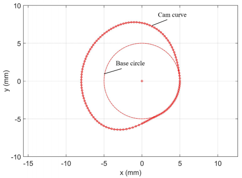
The optimal cam curve is obtained by solving Eq. (26) using the algorithm in Table 1. Moreover, the optimal parameters of cam, i.e., base circle radius and pressure angle are also achieved. The cam size is depended on the base circle; choosing the best base circle radius is thus an important role in cam calculation. The pressure angle of cam is also an important parameter that affects to the transmission cam mechanism. It can be sated that the pressure angle decreases when the base circle radius of the cam increases. Normally, the pressure angle of cam mechanisms is no larger than 30°. Therefore, the optimal values of the base circle radius and the pressure angle must be considered in computing the cam knife-edge follower. Computing the base circle has to satisfy the condition of the pressure angle, i.e., $\Phi \leq 30^{\circ}$. For this, the result of the optimal cam curve is presented in Figure 3, in which the base circle radius is 5mm, and the maximum value of the pressure angle is computed as 29.3619°.
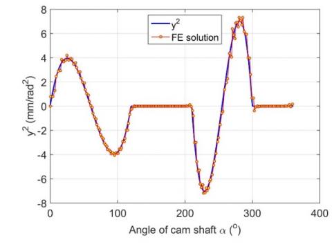
Figure 4 shows the displacement, velocity and acceleration of the cam knife-edge between given transfer function and FE solution. The maximum error between EF solution and given transfer function is 5.4363×10⁻⁵.
Figure 5 depicts the change of the pressure angle $\Phi$ during the cam motion angle in one revolution (a=0÷360°). Values of the pressure angle at all positions of cam satisfy the condition of transmission of the cam mechanism.
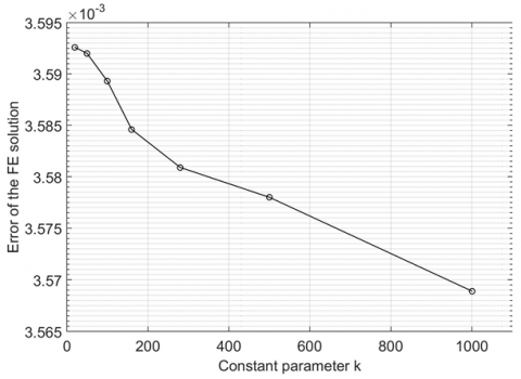
In order to evaluate the constant parameters in cam optimization, Figure 6 describes the relation between the constant parameter k and the error of the EF solution. It is clearly seen that when the value of the constant parameter increases, the accuracy of the FE solution increases. The pressure angle decreases when the constant parameter increases as shown in Figure 7. For this, the lager the value of the constant parameter, the more accurate solution is. Thus, in order to obtain the exact solution, the value of the constant parameter may need to approach the infinity.
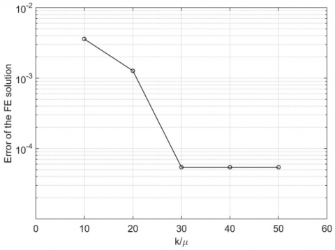
Figure 8 and Figure 9 present the effect of the ratio $k / \mu$ on the accuracy of cam design and the pressure angle. From the observarion of Figure 8, the accuracy of FE solution increases when the ratio $k / \mu$ increases; otherwise, the pressure angle is reduced (see Figure 9). When the ratio $k / \mu$ increases until some values ($k / \mu$=30, 40, 50), the accuracy does not increase, and the pressure angle does not decrease any more (see Figure 9).
Figure 3. Designed cam curve
a) Displacement
b) Velocity
c) Acceleration
Figure 4. Kinematics of cam knife-edge follower
Figure 5. Pressure angle of the cam mechanism
Figure 6. The relation between constant parameter and error of the FE solution
Figure 7. The graph between constant parameter with pressure angle
Figure 8. The effect of k/$\mu$ on the accuracy of FE solution
Figure 9. The effect of k/$\mu$ on the pressure angle
In this study, the procedure of computing the cam knife-edge follower has been given as follows:
After all the above computations, the cam curve is obtained, which considers both the cam size and the pressure angle. For this, the base circle radius is selected to optimal cam size. Moreover, the pressure angle is computed to satisfy the transmission condition of the cam mechanism. Additionally, the effect of constant parameter and the stabilized parameter on the design cam curve has been discussed. From this, the designer can choose the suitable parameters in the computation of cam curves for cam knife-edge follower mechanisms. However, using the potential energy, the constant parameter must choose the large value to obtain the exact solution for the finite element method. With this approach method, the important parameters of the cam knife-edge follower are flexibly the evaluation and optimal design. This is an essential characteristic of the cam design. In future research, this method could explore the application of other related fields in other contexts and the potential limitations of the methodology.
The author would like to thank Thai Nguyen university of Technology for supporting this article.
|
yo |
given transfer function, mm |
|
|
y |
current transfer function, mm |
|
|
ro |
base circle radius, mm |
|
|
a |
coefficients of the polynomial function |
|
|
d |
vector of follower motion direction |
|
|
x1 |
vector horizontal direction |
|
|
x |
desired cam curve |
|
|
C(x) |
current curve |
|
|
Co(x) |
initial curve |
|
|
a1 |
tangent vector of the co-variant on current curve |
|
|
a1 |
tangent vector of the contra-variant on current curve |
|
|
A1 |
tangent vector of the co-variant on given curve |
|
|
n |
normal vector |
|
|
b, r |
vectors |
|
|
B, E |
second-order tensors |
|
|
I |
second-order identity tensor |
|
|
N |
shape functions |
|
|
k |
constant parameter |
|
|
K |
tangent matrix |
|
|
f |
nonlinear equation |
|
|
Greek symbols |
||
|
$\alpha$ |
angle of camshaft, ° |
|
|
$\Pi$ |
design function |
|
|
$\Delta$ |
linearilization |
|
|
$\delta$ |
variation |
|
|
$\mu$ |
stabilized parameter |
|
|
$\Phi$ |
pressure angle, ° |
|
|
Subscripts |
||
|
p |
potential energy |
|
|
s |
stabilized constraint |
|
|
e |
Node of element |
|
[1] Zhou, X., Chen, Z., Zou, P., ping Liu, J., bo Duan, X., yu Li, Q., zi Shen, D. (2020). Kinematics analysis and design method of a new mechanical CVVL system with self-regulation of the valve timing. Mechanism and Machine Theory, 143: 103624.
[2] Zhang, Z., Liu, F., Wang, P., Hu, R., Sun, B. (2017). Methodology to parametric design of cam profile for electronic unit pump. Energy, 139: 170-183. https://doi.org/10.1016/j.energy.2017.07.142
[3] Jamkhande, A.K., Tikar, S.S., Ramdasi, S.S., Marathe, N.V. (2012). Design of high speed engine's cam profile using B-spline functions for controlled dynamics. SAE Technical Paper, 2012(28): 0006. https://doi.org/10.4271/2012-28-0006
[4] Lin, D.Y., Hou, B.J., Lan, C.C. (2017). A balancing cam mechanism for minimizing the torque fluctuation of engine camshafts. Mechanism and Machine Theory, 108: 160-175. https://doi.org/10.1016/j.mechmachtheory.2016.10.023
[5] Qin, W., Chen, Y. (2014). Study on optimal kinematic synthesis of cam profiles for engine valve trains. Applied Mathematical Modelling, 38(17-18): 4345-4353. https://doi.org/10.1016/j.apm.2014.02.015
[6] Chowdhury, A.R. (2020). Design analysis of spring and cam follower mechanism. International Research Journal of Engineering and Technology (IRJET), 7(6): 3121-3124. http://dx.doi.org/10.13140/RG.2.2.12946.68802
[7] Hsieh, J.F. (2014). Design and analysis of indexing cam mechanism with parallel axes. Mechanism and Machine Theory, 81: 155-165. https://doi.org/10.1016/j.mechmachtheory.2014.07.004
[8] Sun, S., Qiao, Y., Gao, Z., Huang, C. (2022). Research on machining error analysis and traceability method of globoidal indexing cam profile. Machines, 10(3): 219. https://doi.org/10.3390/machines10030219
[9] Norton, R.L. (2003). Design of machinery. Mcgraw-hill.
[10] Sarma, N., Barua, P.B., Kalita, D. (2015). Optimization model for disc cam flat faced follower mechanism. International Journal of Engineering Trends and Technology, 29: 6-11. https://doi.org/10.14445/22315381%2FIJETT-V29P202
[11] Patel, H.D.P.V. (2010). Computer aided kinematic and dynamic analysis of cam and follower. In Proceedings of the World Congress on Engineering, Vol. 2.
[12] Shin, J.H., Kwon, S.M., Nam, H. (2010). A hybrid approach for cam shape design and profile machining of general plate cam mechanisms. International Journal of Precision Engineering and Manufacturing, 11(3): 419-427. https://doi.org/10.1007/s12541-010-0048-6
[13] Hong-Sen, Y., Wen-Teng, C. (1999). Curvature analysis of spatial cam-follower mechanisms. Mechanism and Machine Theory, 34(2): 319-339. https://doi.org/10.1016/S0094-114X(98)00038-X
[14] Kiran, T., Srivastava, S.K. (2013). Analysis and simulation of cam follower mechanism using polynomial cam profile. International Journal of Multidisciplinary and Current Research, 210-217.
[15] Liang, Z., Huang, J. (2014). Design of high-speed cam profiles for vibration reduction using command smoothing technique. Proceedings of the Institution of Mechanical Engineers, Part C: Journal of Mechanical Engineering Science, 228(18): 3322-3328. https://doi.org/10.1177/0954406214528321
[16] Luo, H., Yu, J., Li, L., Huang, K., Zhang, Y., Liao, K. (2022). A novel framework for high-speed cam curve synthesis: Piecewise high-order interpolation, pointwise scaling and piecewise modulation. Mechanism and Machine Theory, 167: 104477. https://doi.org/10.1016/j.mechmachtheory.2021.104477
[17] Tsay, D.M., Huey Jr, C.O. (1993). Application of rational B-splines to the synthesis of cam-follower motion programs. Journal of Mechanical Design. Trans. ASME, 115(3): 621-626. https://doi.org/10.1115/1.2919235
[18] Nguyen, T.N., Kurtenbach, S., Hüsing, M., Corves, B. (2019). A general framework for motion design of the follower in cam mechanisms by using non-uniform rational B-spline. Mechanism and Machine Theory, 137: 374-385. https://doi.org/10.1016/j.mechmachtheory.2019.03.029
[19] Sateesh, N., Rao, C.S.P., Janardhan Reddy, T.A. (2009). Optimisation of cam-follower motion using B-splines. International Journal of Computer Integrated Manufacturing, 22(6): 515-523. https://doi.org/10.1080/09511920802546814
[20] Sun, C.Q., Ren, A.H., Sun, G.X. (2011). Optimum design of motion curve of cam mechanism with lowest maximum acceleration. In Applied Mechanics and Materials. Trans Tech Publications Ltd, 86: 666-669. https://doi.org/10.4028/www.scientific.net/AMM.86.666
[21] Li, Z.J., Li, F., Wang, H.J. (2014). A study on conjugate cam beating-up mechanism. In Applied Mechanics and Materials. Trans Tech Publications Ltd, 668: 134-137. https://doi.org/10.4028/www.scientific.net/AMM.668-669.134
[22] Yang, L.I., Guoguang, J.I.N., Zhan, W.E.I., Yanyan, S. (2020). Dynamic characteristics analysis of conjugate cam beating-up mechanism of rapier loom. In 2020 3rd World Conference on Mechanical Engineering and Intelligent Manufacturing (WCMEIM). IEEE, pp. 823-830. https://doi.org/10.1109/WCMEIM52463.2020.00176
[23] Ming, C., Chi, X., Sun, Z., Sun, Y. (2022). Design of electronic cam for lower hook mechanism of fishing net-weaving machine based on polynomial fitting. Textile Research Journal, 92(11-12): 1748-1759. https://doi.org/10.1177/00405175211068784
[24] Alaci, S., Ciornei, F., Filote, C. (2015). Rotating cam and knife edge follower mechanism optimisation from cam curvature constraints. In Applied Mechanics and Materials. Trans Tech Publications Ltd, 809: 598-603. https://doi.org/10.4028/www.scientific.net/AMM.809-810.598
[25] John, U., Gordon, P., Joseph, S. (2017). Theory of Machines and Mechanisms.
[26] Myszka, D.H. (1999). Machines and mechanisms: applied kinematics analysis. Prentice Hall.
[27] Sauer, R.A. (2016). A contact theory for surface tension driven systems. Mathematics and Mechanics of Solids, 21(3): 305-325. https://doi.org/10.1177/1081286514521230