Enhancing Image Classification Through a Hybrid Approach: Integrating Convolutional Neural Networks with Hidden Markov Mod

A fundamental problem in computer vision is image classification, which is labeling or categorizing images based on their visual characteristics. By accurately collecting spatial patterns and learning to distinguish features from images, although it can also be used with one-dimensional and tridimensional data, CNNs, or convoluted neural networks, are a specialized sort of neural network model designed to operate with bidimensional image data. These networks are able to learn to extract local characteristics, that is, structures that repeat themselves throughout the image. CNNs have shown exceptional effectiveness in image categorization. CNNs are widely used in various applications, such as object detection, image classification, and facial recognition, due to their ability to learn and extract meaningful features from images [1]. The use of deep learning algorithms like CNNs has revolutionized the field of computer vision and led to significant advancements in image classification tasks. With the help of feature extraction and dimensionality reduction, the representations from the input images.

To build the new CNN architectures into the IT vision domain [2-6]. Dehghan et al. [7] utilized CNN provides a more sophisticated method for classifying images and detecting things. There are sophisticated numbers in this technology. The terms you desire for a memento are used by artificial intelligence and autonomous applications. CNNs are helpful, particularly in situations with a lot of data, image classification, etc. Their augmented usage across various industries can be attributed to their exceptionally precise outcomes and forecasts. HMMs are frequently used to predict the future behavior of individual elements. The HMM is based on the theory that an element's future behavior is determined by its past behavior as well as the behavior of other nearby elements. The HMM can be used to understand the relationships between the elements in an ensemble of data as well as predict how individual elements will behave in the future.

HMMs, on the other hand, are frequently used for sequential data modeling and have historically been used in areas like speech recognition or natural language processing [8]. The goal is to use the sequential modeling capabilities of HMMs to capture dependencies in the derived features from CNNs [9], improving the classification's accuracy and discriminative ability. The other tactic is to compile all of the data in order to apply models that are more capable of deep learning, but at the expense of losing track of individual behavior information. This memory's hypothesis is that, despite the second strategy's lower performance, it still provides useful information and that using both strategies together can improve overall performance and mitigate the issue of the individualized strategy's potential data shortage.

The hybrid HMM-CNN [10] technique takes advantage of the advantages of both models to overcome the drawbacks of standalone CNNs by merging these two potent algorithms.

Researchers have recently looked into the possible advantages of a hybrid approach for picture classification that combines the advantages of both HMMs and CNNs [11].

This hybrid approach tries to combine, in a beneficial way, the temporal modeling provided by HMMs [12] and the spatial analysis provided by CNNs [13, 14]. CNN components extract complex patterns and high-level Following that, these features are fed into an HMM, which simulates the temporal correlations between the collected features and enables the use of sequential data for better categorization.

This hybrid design potentially opens up a path for improved image classification performance, especially in applications like video analysis or image recognition where temporal dependencies are critical.

Throughout this investigation, we will delve into the precise procedures, techniques, and considerations associated with putting a hybrid HMM-CNN [15] approach to use in building an image classification system. We will look at how the sequential modeling skills of HMMs [16] can be paired with the feature extraction capabilities of CNNs [17] to produce results in image classification that are more reliable and accurate. In this work, CNN was used to extract the characteristics, while HMM was employed to classify the images.

In this work, we propose a hybrid method that combines HMMs and CNNs for image classification. The CNN [18] is used to extract features from the images, while the HMM is used to model the spatial dependencies between adjacent image pixels [19]. The resulting classification performance is evaluated on a skin layer dataset, and the results show that the proposed method outperforms other state-of-the-art methods. The rest of the paper is organized as follows: Section 2 provides a brief overview of CNNs and HMMs; Section 3 describes the proposed hybrid method; Section 4 presents the experimental results; and Section 5 concludes the paper.

The results of these studies suggest that the hybrid CNN-HMM model can be an effective approach for image classification, leveraging the strengths of both CNNs and HMMs. The CNN can extract features from the image that are relevant to the task of classification, while the HMM can model the spatial relationships between adjacent pixels and identify boundaries between different regions in the image.

However, the effectiveness of the hybrid model depends on various factors, including the complexity of the image, the number of classes, and the quality of the training data. Further research is needed to evaluate the performance of the hybrid CNN-HMM model for different types of images and applications.

In this paper, I will describe the architecture of the CNN model. I have developed it for image classification and demonstrated its application on the CIFAR-10 dataset. The model is implemented using the Keras API, which is built on top of Tensor Flow. The architecture of the model consists of several convolutional layers, followed by batch normalization and max-pooling layers, which help to improve the stability of the training process and reduce overfitting. Dropout is also implemented to further prevent overfitting. The fully connected layer at the end of the model has a large number of neurons, which increases the model's capacity and allows it to learn more complex features. The model is trained using the Adam optimizer and the categorical cross-entropy loss function. By training the model on the CIFAR-10 dataset for multiple epochs, the model learns to accurately classify images into 10 different classes. Overall, the combination of the CNN architecture, batch normalization, dropout, and optimization techniques make the model highly effective at image classification tasks.

3.1 Software and tools

3.1.1 Python

Python is a high-level, interpreted programming language known for its simplicity, readability, and versatility. It was created by Guido van Rossum and first released in 1991. Python's design philosophy emphasizes code readability, making it easy for developers to express concepts clearly and concisely. One of Python's defining features is its clean and intuitive syntax, which allows programmers to write code more naturally and expressively. This readability not only enhances developer productivity but also facilitates collaboration among teams. Python provides a vast standard library that offers a wide range of modules and functions for various tasks, such as file handling, networking, web development, data manipulation, and more. Additionally, Python has a thriving ecosystem of third-party libraries and frameworks that extend its capabilities, enabling developers to tackle specialized domains like machine learning, scientific computing, and data analysis. Python's interpreted nature allows for rapid development and prototyping. It supports multiple programming paradigms, including procedural, object-oriented, and functional programming, giving developers the flexibility to choose the approach that best suits their needs. The strength of Python is its cross-platform compatibility, enabling code to run seamlessly on different operating systems. This portability makes Python a popular choice for developing applications that need to work across various platforms and environments. Python has a large and supportive community that contributes to its growth and development. The community provides extensive documentation, tutorials, and forums where programmers can seek help, share knowledge, and collaborate on open-source projects. In summary, Python is a versatile programming language that prioritizes simplicity, readability, and ease of use. Its extensive standard library, diverse ecosystem, cross-platform compatibility, and supportive community make it a popular choice for a wide range of applications and skill levels.

3.1.2 CNN’s architecture

qqjie_tu_20240229134622.png

Figure 3. CIFAR-10 dataset

Table 1. The architecture of the used model for my test

The studied model consists of a total of 18 layers, including 6 convolutional layers, 3 max-pooling layers, 6 batch normalization layers, 3 dropout layers, 1 flattening layer, and 2 dense layers. The input image, which has a size of 32x32 pixels, is passed through these layers sequentially to classify it into one of the 10 classes in the dataset. This table displays a comprehensive summary of the model's architecture, providing detailed information about each layer and its corresponding parameters. Please refer to the table for a visual representation of the model's architecture.

Figure 3 shows the detailed architecture (summary) of the Model: "sequential"

This table (Table 1) shows the detailed architecture (summary) of the model: "sequential".

3.1.3 Hardware

The hardware utilized throughout the implementation of the entire project is described in Table 2.

Table 2. The hardware used to run the tests

3.2 Data set

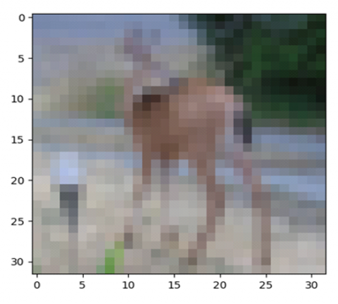
Researchers and practitioners often utilize the CIFAR-10 dataset to evaluate and compare the performance of different image classification algorithms and models. It serves as a benchmark for assessing the accuracy and generalization capabilities of machine learning models in classifying images from different categories. The CIFAR-10 dataset has contributed to advancements in computer vision and deep learning research. It has been used to train and evaluate various state-of-the-art models, including CNNs, to achieve high accuracy in image classification tasks. To initiate my tests, I began by visualizing a randomly selected sample from the dataset. Please refer to Figure 4 for an illustration of this random sample. In this code, we are going to build a CNN model that can classify images of various objects. We have 10 classes of images, such as: airplane, automobile, bird, cat, deer, dog, frog, horse, ship, and truck.

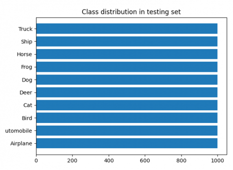
Upon executing the code, some results were attained. Figure 5 provides a summary of the class distribution in the training set, while Figure 6 depicts the class distribution.

qqjie_tu_20240229134910.png

Figure 4. A random sample from the dataset

qqjie_tu_20240229141156.png

Figure 5. Class distribution in the training set

qqjie_tu_20240229142343.png

Figure 6. Class distribution in the testing set

The testing set is presented below.

Training Section

The provided lines represent the training and validation progress of a model over 50 epochs. Throughout the training process, the model's performance is evaluated using various metrics such as loss, accuracy, precision, and recall.

In the beginning, during the first epoch, the model achieved a relatively low accuracy of 0.4095 on the training set, indicating that it initially struggled to make accurate predictions. However, there was a notable precision of 0.6303, suggesting that when the model made predictions, they were relatively reliable. The recall, which measures the model's ability to identify positive instances correctly, was at 0.1953, indicating room for improvement.

As the training progressed, the model's performance gradually improved. By the 50th epoch, the model achieved a significantly higher accuracy of 0.8755 on the training set, indicating that it learned to make more accurate predictions over time. Both precision (0.9091) and recall (0.8459) were relatively high, suggesting that the model was effectively identifying and classifying positive instances.

Overall, the model's performance progressed positively throughout the training process, demonstrating an increasing ability to make accurate predictions and classify positive instances.

In Table 3, we present the performance of the criteria.

Table 3. The values of criteria to run the tests

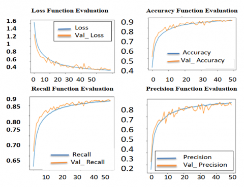
Accuracy and Model Loss

Figure 7 suggests that the model is learning and acquiring more information over time. Consequently, the training loss decreases at a faster rate than the validation loss, indicating improved performance on the training data. The widening gap between the training and validation curves may indicate potential overfitting, necessitating techniques to enhance generalization.

qqjie_tu_20240229140353.png

Figure 7. Test accuracy and model loss plots

In the confusion matrix, we see that the truck class is misclassified for the different classes used in this paper.

As an example, the model classified the images of birds, cats, and trucks and misclassified the images of dogs, frogs, and deer (Figure 8).

qqjie_tu_20240229141037.png

Figure 8. The confusion matrix of the model

The confusion matrix is a valuable tool for evaluating the performance of a model as it provides insights into the true positive, true negative, false positive, and false negative metrics. In Figure 13, the arrangement of these metrics for each class is depicted, offering a clear visual representation of the model's performance in terms of correct and incorrect classifications.

Error Rate

Figure 9 depicts the error rate of the classified and misclassified images by the trained model. Upon observation, it can be inferred that the model has achieved a satisfactory level of accuracy, as the misclassification rate is less than one-fourth of the entire dataset.

qqjie_tu_20240229141111.png

Figure 9. The error rate of the model

Accuracy

Upon completing the tests, the model demonstrated its ability to accurately classify images, achieving a test accuracy of 87.09%. This indicates the model's proficiency in accurately predicting the correct classes for the test dataset.