Ayam M. Abbass*![]() | Basma Jumaa Saleh
| Basma Jumaa Saleh![]() | Liqaa Saadi Mezher
| Liqaa Saadi Mezher![]()
This article is part of the Special Issue the Impact of AI on Decision-Making
© 2024 The authors. This article is published by IIETA and is licensed under the CC BY 4.0 license (http://creativecommons.org/licenses/by/4.0/).
OPEN ACCESS
This study aims to improve the control of robotic knee flexion during walking, with a particular emphasis on enhancing mobility and rehabilitation for patients with mobility problems. The objective is to develop a high-performance controller by integrating the Desired Optimal Controller (DOC)-based Multivariable Model Reference Adaptive Control (MRAC) algorithm with sophisticated optimization techniques. This study notably combines the Whale Optimization Algorithm (WOA) with a novel approach called Combined WOA-KHO to precisely optimize controller parameters. The technique provides a thorough explanation of the construction of the DOC-based MRAC algorithm, which employs a second-order transfer function for the reference model. This study emphasizes the inclusion of adaptive gains, the structural characteristics of the best controller, and the implementation of a deep neural network (DNN)-PID control system utilizing a Multi-Layer Feed-Forward Neural Network (MLFNN). In addition, this text elaborates on the optimization strategies, namely the employment of the Whale Optimization Algorithm (WOA) and the Combined WOA-KHO algorithm. The simulation results clearly demonstrate the gradual improvement of the system's performance, providing evidence for the effectiveness of the suggested DOC-based MRAC algorithm and the optimization approaches. An extensive examination of the system's response characteristics, such as settling time, rising time, and steady-state error, is performed using several simulations. A performance comparison is implemented between three optimization algorithms: Genetic Algorithm (GA), Particle Swarm Optimization (PSO), and WOA. The study finds that using all three algorithms together significantly improved the gait control of a robotic knee system, outperforming the results obtained from traditional algorithm.
robotic human knee, desired optimal controller (DOC), multivariable model reference adaptive control (MRAC) algorithm, whale optimization algorithm (WOA), krill herd algorithm (KHA)
Recently, there is a surge in robotics research focused on observing how humans move, abnormal walking patterns, and developing models and limb structures that mimic human capabilities [1]. As growing in the number of people suffering from limb loss due to accidents, illnesses, injuries, and disasters, there is a growing urgency to find techniques to retrieve their physical abilities. This is important for ensuring their well-being and ability to lead independent lives [2]. The robotic knee prosthesis is an important part to help people walk. It operates by controlling the position of the lower leg, generating the necessary knee force, and reducing movement during the leg swing. This helps to stabilize the lower limb and allows for walking [2].
Globally, about 1.1 billion people suffer from disability and technology that helps people with disabilities can improve their lives significantly. It helps them to be more independent and involved in society [3]. Exoskeletons are designed to help walking implement diverse control strategies on lower limbs. Powered lower-limb orthotic devices, commonly referred to as powered exoskeletons, are widely recognized as rehabilitation and gait assistance tools [4].
To enable the functionality of a robotic knee prosthesis, a prosthesis controller module receives sensor readings from joint encoders, force sensors, and an inertial measurement unit. It utilizes this information to transmit commands to the prosthesis device, such as the desired motor position or torque [5]. The integration of physical hardware, software control algorithms, and user interaction poses several challenges in effectively assisting individuals with impaired locomotion using robotic devices. Overcoming these challenges involves enabling users to employ various gait patterns and developing robust evaluation methods to assess the effectiveness and performance of assistive devices [6].
Following femoral amputation, numerous active prostheses have been developed to rehabilitate gait function, capable of producing and controlling knee torque. Various strategies have been proposed to control active femoral prostheses. For instance, Rifaï et al. [7] presented an adaptive control approach for knee joint orthosis considering a user's effort, Chevalier et al. [8] discussed a theoretical model for shank movement around the knee joint and employed two design techniques, model-based design, and auto-tuning, to design a PID controller for controlling the shank angle.
Furthermore, Rifaï et al. [7] developed an adaptive sliding mode controller based on super-twisting for knee joint orthosis. Their approach incorporated a human-driven model, Bkekri et al. [9] proposed a sliding mode controller based on the theory of Lyapunov stability.
Considering a mathematical model of a nonlinear system combining human shank dynamics and knee joint orthosis, Kohli et al. [10] designed a feedback linearization controller. Khalaf et al. [11] proposed a design and control method by experimentally evaluating the regenerated energy across a femoral prosthesis during the swinging phase of a gait cycle.
In recent years, researchers have shown great interest in nature-inspired algorithms. Swarm intelligence (SI) algorithms have gained prominence. These algorithms emulate the operation of natural systems, such as animal or plant behavior, to develop effective optimization techniques plants [12, 13]. Particle swarm optimization (PSO) [14], artificial bee colony algorithm (ABC) [15], ant colony optimization (ACO) [16], grey wolf optimization (GWO) [17], krill herd algorithm (KHA) [18], brainstorm optimization (BSO) [19], and whale optimization algorithm (WOA) [20] are all examples of popular SI algorithms.
The Whale Optimization Algorithm (WOA) [20] is a new kind of optimization algorithm. The natural hunting techniques of humpback whales served as inspiration for this algorithm. WOA uses three operators—"encircle prey," "research prey," and "attack prey"—to track down its meals. WOA has undergone significant change. These studies can be broken down into two broad categories. Using the WOA to solve real-world problems is one of them. The other is to implement measures that enhance WOA's functionality [21].
Another swarm intelligence search algorithm inspired by the coordinated foraging behavior of krill is known as the "Krill Herd" (KH) algorithm [18]. Individual krill navigate a three-dimensional region in search of nearby food and a dense herd, as part of a population-based strategy involving a very large number of krill. With KH as an optimization algorithm, the distance of a krill from its food source is treated as a design variable. There are three types of algorithms that can be compared to the KH algorithm: (1) Evolutionary algorithms (2), a bacterial foraging algorithm, and (3), swarm intelligence [22, 23].
In order to underscore the pragmatic ramifications of WOA, a case study [24] concerning the real-time PID controller optimization of a micro robotics system demonstrates WOA's exceptional performance relative to Grey Wolf Optimization. The study provides evidence that WOA exhibits superior performance compared to alternative methods, as determined by its ISTES cost function, which decreases error by 47.5%. WOA is suggested by these empirical results for adjusting PID parameters in micro robotic systems.
Previous research does not address the nonlinearity of robotic knee flexion during walking, with a particular emphasis on enhancing mobility and rehabilitation for patients. Therefore, in this context, this paper aims to address the design of an optimized Desired Optimal Controller (DOC)-based multivariable Model Reference Adaptive Control (MRAC) algorithm for robotic human knee flexion during gait. This algorithm assists the robotic knee joints to achieve better performance to match how people walk and their body's needs. Gives help to people who have moving problems to feel natural and move in an efficient manner. The aim is to design a controller that exhibits fast rise time with no overshoot and the steady-state error approaches zero. By incorporating concepts from DOC and MRAC, it will give these desired characteristics smoothness, energy efficiency, stability, and compatible with the patterns of the user's gait. Hence, the objective of the proposed investigation is to:
1. Maximizing the Performance of Robotic Knee Joints:
·Design of a control system which ensures the response of the robotic knee joints to be appropriate for different inputs and conditions.
·Enhance the capacity to adapt to various locomotion patterns and the physiological circumstances.
2. Attaining Precise Control Attributes:
·Make sure that the flexion of the knee is seamless and with no overshoot.
·Achieve a rapid onset of motion and eradicate steady-state error while walking.
3. Desired Optimal Control and MRAC Integration:
·Blend the tenets of Model Reference Adaptive Control and Desired Optimal Control.
4. Improvements to Controller Attributes:
·Ensure the energy efficiency, fluidity, and stability of the control system.
·Customized assistance can be achieved by aligning the controller with the user's unique locomotion patterns.
5. Development and Validation of Algorithms:
·Construct a comprehensive MRAC algorithm utilizing DOC.
·Conduct experiments and simulations to evaluate the efficacy of the algorithm.
6. Investigation of Methods for Combined Optimization:
·Explore the potential for integration between WOA and KHO.
·Evaluate the advantages of integrating WOA-KHO in contrast to conventional optimization algorithms.
This paper will further explore the development, simulation, and experimental validation of the algorithm in the following sections. By doing so, it will make a valuable contribution to the field of robotic knee prosthesis technology, which aims to enhance gait assistance and rehabilitation.
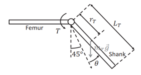
Figure 1. The biomedical model of tibial movement [8]
To regulate the motion of the tibial in the knee joint, a system transfer function is employed to derive a two-dimensional model. Particular attention is devoted to the dynamics occurring in the sagittal plane. This deliberate simplification is based on the valid assertion that the magnitudes of motions in the coronal plane are relatively lesser than those observed in the sagittal plane. Figure 1 depicts the biomedical model of tibial movement.
The biomechanical model consists of the upper leg segment (femur) and the lower leg segment (tibia and fibula, collectively known as the shank). A revolute joint connects these segments. A torque denoted by T is applied at the knee joint, which serves as the input for this biomechanical model. In this biomedical model, LT represents the shank's length, rT is the distance between the center of the shank's mass and the axis of the knee joint, while mT denotes the shank's mass, and g represents a gravitational constant. In this work, the values of the biomedical model's parameters are taken from [8], where LT=0.435 m; mT=3.72 kg, and rT=0.188 m.
The range of motion of the shank is represented by the angle, which spans 90°. This enables the shank to move from a vertical to a horizontal position. The angle =0° corresponds to the range's midpoint, which is 45° s off the vertical line. Consequently, =45° indicates complete leg extension. The angle denotes this system's output. The parameters for the biomedical model are taken from [8] and defined in Table 1.
Table 1. The parameter for the biomedical model
|
Symbol |
Description |
Values |
|
B |
Viscous Damping |
6.75 Nms/rad |
|
IT |
Inertia around a knee joint |
0.44 Kgm2 |
|
K |
Stiffness of the knee joint |
44.22 Nm/rad |
|
g |
Acceleration due to gravity creates a nonlinear torque |
9.8 m/s2 |
The system torque contributions include gravitational torque, shank inertia torque, viscous damping torque, joint rigidity torque, and applied torque T(t). Considering the directionality of each torque, we can derive the following Eq. (1) by adding them [8]:
$\begin{gathered}I_T \frac{d^2 \theta(t)}{d t^2}+\mathrm{B} \frac{d \theta(t)}{d t}+\mathrm{K} \theta(t)+m_T g r_T \sin (\theta(t)+\left.45^{\circ}\right)=\mathrm{T}(\mathrm{t})\end{gathered}$ (1)
where, IT is the shank's inertia around the knee joint, while B is the knee joint's viscous damping coefficient, and k represents the stiffness of the knee joint. The Equation of motion must be linearized around an equilibrium point to determine the system's transfer function. In this instance, the equilibrium point chosen corresponds to the condition in which θ*=0°. Simplify the Eq. (1) as specified in [8] to get the linear Eq. (2) for the model:
$I_T \ddot{\theta}+\mathrm{B} \dot{\theta}+\mathrm{K} \theta(t)+\frac{\sqrt{2}}{2} m_T \cdot g r_T \cdot \theta(t)=\mathrm{T}(\mathrm{t})$ (2)
where, $\theta, \dot{\theta}, \ddot{\theta}$ represent the angular distance, velocity, and acceleration of the plant motion. For Eq. (2), which takes the Laplace transform and assumes initial conditions of zero, the transfer function for this model is given [8]:
$\frac{\theta(s)}{T(s)}=\frac{1}{I_T s^2+B s+\left(K+\frac{\sqrt{2}}{2} m_T \cdot g \cdot r_T\right)}$ (3)
By substituting the system's parameters in Eq. (3) as specified in [8], we will get the system transfer function in Eq. (4):
$\mathrm{TF}(\mathrm{s})=\frac{1}{0.44 s^2+6.75 s+49.07}$ (4)
This transfer function corresponds to a second-order system with a damping ratio (ζ)=0.72 and natural frequency (ωn)=10.54.
This paper provides a comprehensive overview of WOA and KHA, shedding light on their significance and potential applications in solving optimization problems. The subsequent sections will delve into the details of these algorithms, elucidating their mechanisms and showcasing their contributions to the advancement of optimization techniques.
3.1 The whale optimization algorithm (WOA)
The key algorithm is inspired by the habits of whales. WOA's basic performance consists of three stages: prey encirclement, bubble-net assault, and prey discovery. In what follows, it will discuss the mathematical models of three distinct strategies [12, 20, 21]:
Cascading its victim The humpback whales encircle their prey once they identify its location. In the absence of prior knowledge regarding the location of the optimal design in the search space, the WOA algorithm operates under the assumption that the current best candidate solution is either the target prey or is near the optimum, thereby indicating its suitability as the search agent. As a result, the remaining agents will endeavor to revise their stances regarding this agent. The other search agents update their locations by moving onward to the best-fitted agent which is followed by the below equations:
$\vec{Ð}=\left|\vec{ Ç } \cdot \overrightarrow{X^*}(t)-\vec{X}(t)\right|$ (5)
$\vec{X}(t+1)=\overrightarrow{X^*}(t)-\overrightarrow{\text { Á }} \cdot \vec{Ð}$ (6)
where, $X^*, \vec{X}$, and $t$ represent the location coordinate of the optimal solution, the current each iteration, and the position vector format correspondingly. Coefficient vectors, denoted as $\vec{ Á }$ and $\text { Ç }$ are known as coefficient vectors and calculated by using the below equations:
$\vec{Á }=2 \vec{á} \cdot \vec{r}-\vec{á}$ (7)
$\vec{Ç}=2 \vec{r}$ (8)
where, $\vec{r}$ represents the random vector within the range $[0,1]$, and with each iteration, the value of $\vec{á}$ decreases linearly from 2 to 0.
(b) Exploitation stage (i.e., the bubble-net attack); the two operations comprising the exploitation stage.
(1) The implementation of a diminishing encircling mechanism involves the reduction of a value as specified in Eq. (4). Note that $\vec{á}$ is a random value between $[-\vec{á}, \vec{á}]$.
(2) The spiral update positional method is utilized to compute the distance separating the cetacean and its prey. The following spiral equation is used to simulate the helix-shaped motion:
$\vec{X}(t+1)=\overrightarrow{\mathrm{Ð}}^l e^{b l} \cdot \cos (2 \pi l)+\overrightarrow{X^*}(t)$ (9)
In the given interval [−1, 1], denoted as "l," a random number, and "b" a constant. A probability of 50% is postulated regarding the selection between the spiral model and the shrinking encircling mechanism. The mathematical model is therefore expressed as follows:
$\vec{X}(t+1)=\left\{\begin{array}{c}\overrightarrow{X^*}(t)-\vec{Á} \cdot \vec{\ominus}, \quad P<0.5 \\ \vec{Ð}^l e^{b l} \cdot \cos (2 \pi l)+\overrightarrow{X^*}(t), \quad \mathrm{P} \geq 0.5\end{array}\right.$ (10)
The symbol $P$ denotes a number chosen at random from a uniform distribution.
(c) Stage of exploration (i.e., pursuit of the prey). The exploration for target method utilizes a variation of $\vec{Á}$ that is either greater than 1 or less than −1. As of now, during the exploitation phase, update the location of a search agent. The mathematical model shown below is employed to conduct a global search for $|\vec{Á}|>1$.
$\overrightarrow{\mathrm{Ð}}=\left|\vec{Ç} \cdot \vec{X}_{\text {rand }}-\vec{X}\right|$ (11)
$\vec{X}(t+1)=\vec{X}_{\text {rand }}-\overrightarrow{\mathrm{Á}} \cdot \stackrel{\rightharpoonup}{\mathrm{Ð}}$ (12)
where, $\vec{X}_{\text {rand }}$ is a random location vector which is chosen from existing population.
Algorithm 1 shows the pseudo-code of the original WOA algorithm.
WOA
Initialize a population of n random whales or search agents Xi (i=1, 2, 3, …, n).
Evaluate each search agent B the best search agent.
While (t< max - epoch)
for each search agent in the population
Update WOA parameters $(\vec{á}, \vec{Á}, \vec{Ç}, l, P)$
if $(\mathrm{P}<0.5)$
if $(|\vec{Á}|<\boldsymbol{l})$
Update the current search agent by $\vec{X}(t+1)=B-\vec{Á} \cdot \vec{Ð}$
else if $(|\bar{Á}| \geq l)$
select a random search agent $\left(\vec{X}_{\text {rand }}\right)$
update the current search agent by $\vec{X}(t+1)=\left(\vec{X}_{\text {rand }}\right)-\vec{Á} \cdot \vec{Đ}$
end if
else if $(P \geq 0.5)$
Update the current search agent by $\vec{X}(t+1)=\vec{Ð}^l \boldsymbol{e}^{\boldsymbol{b} \boldsymbol{l}} \cdot \cos (2 \pi \boldsymbol{l})+B$
End if
End for
Evaluate the search agent
Update B if there is the better solution in the population
T=t+1
End while
Return B
3.2 Krill herd algorithm (KHA)
The KHA was originally suggested by Gandomi et al. [18] to model the movement of krill in the ocean. Local and global search are balanced adequately, which is one of the primary benefits of KHA that improves its discovery capability. Upon calculating the objective functional for every krill, this algorithm selects the finest krill [25]. The input layer of the krill herd algorithm is the krill position, and the objective function is sustenance. As shown in Eq. (13), the position of each krill $\left(\mathcal{V}_{\mathrm{ɍ}, i}^{i t r}\right)$ in its life cycle is determined by the factor of induction, the factor of foraging, and the factor of diffusion [22, 23, 25-29] by the following equations:
$\mathcal{V}_{\mathrm{ɍ},i}^{i t r}=\mathcal{V}_{\text {induction}, i}^{i t r}+\mathcal{V}_{\text {foraging}, i}^{i t r}+\mathcal{V}_{\text {diffusion}, i}^{i t r}$ (13)
The factor of induction $\left(\mathcal{V}_{\text {induction}, i}^{\text {itr }}\right)$: The motion of each krill as follows:
$\mathcal{V}_{\text {induction}, i}^{i t r}=\alpha_{\text {induction}, i} \mathcal{V}_{\text {induction}, i}^{\max }+\omega_i \mathcal{V}_{\text {induction}, i}^{i t r-1}$ (14)
where, $\mathcal{V}_{\text {induction}, i}^{\max }$ is the utmost forced speed produced in the absence of other krill, $\mathcal{V}_{\text {induction}, i}^{i t r-1}$ is the last forced activity, ωi is the moment of inertia of the forced motion [0-1], and αinduction,i is the start of the forced move, according to Eq. (15):
$\alpha_{\text {induction,i }}=$$\alpha^{\text {local }}{ }_{\text {induction,i }}+$$\alpha^{\text {target }}{ }_{\text {induction,i }}$ (15)
The local influence given by i neighboring krill is denoted by $\alpha_{\text {local }}^{\text {induction,} \mathrm{i}}$, and the target direction effect formed by $\alpha^{\text {target }}{ }_{\text {induction, i}}$ the ideal krill individual position is denoted by i et.
The factor of foraging $\left(\mathcal{V}_{\text {foraging}, i}^{i t r}\right)$: Each krill adjusts its position based on where it has found food recently and in the past as:
$\mathcal{V}_{\text {foraging}, i}^{\text {itr }}=\mathcal{V}_f \beta_{\text {foraging}, i}+\omega_f \mathcal{V}_{\text {foraging}, i}^{\text {old }}$ (16)
$\mathcal{V}_f$ is the foraging velocity, $\beta_{\mathrm{foraging}, i}$ is the foraging motion their source, $\omega_f$ is the foraging inertial weight between $[0,1]$, and $\mathcal{V}_{\text {foraging,} i}^{\text {old }}$ is the last foraging activity.
$\beta_{\mathrm{foraging}, i}=\beta_{\text {foraging}, i}^{\text {food}}+\beta_{\mathrm{foraging}, i}^{\text {best}}$ (17)
$\beta_{\mathrm{foraging}, i}^{\text {food }}$ stands for i's interest in food, and $\beta_{\mathrm{forag}}^{\text {best}}$ stands for i's interest in being in peak physical condition.
The factor of diffusion ($\mathcal{V}_{\text {diffusion}, i}^{\text {itr}}$): The population's variation is guaranteed by a standard random operator, as in the case of random diffusion:
$\mathcal{V}_{\text {diffusion}, i}^{i t r}=\mathcal{V}^{\max } \delta$ (18)
where, $\mathcal{V}^{\max }$ is the maximum rate of diffusion, δ is a uniformly distributed random vector, and the matrices it generates are numbers in the interval [1, 1]. Combining these three patterns, we can determine an individual krill's location vector from t-to-t Dt by solving Eq. (19) [28]:
$x_i^{i t r+1}=X_i^{i t r}+$$Ḉ_{ɍ, i}^{i t r}$$\times \sum_{j=1}^S\left(U_j-L_j\right)$ (19)
The krill's position at time $\mathrm{t}$ is denoted by $X_i^{i t r}$, and at next time by $\mathcal{X}_i^{i t r+1}$. The maximum and bottom bounds of the variables $\mathcal{U}_j$ and $L_j$, the overall collection of parameters $\mathrm{S}$, and the characteristic of the interval [0,2] are given by $\mathcal{U}_j$ and $L_j$, respectively.
KHA: Idealizing the mobility properties of the krill individuals allows for the creation of a wide variety of algorithms. The following is a high-level overview of the KH algorithm.
Data Structures—Simple Bounds Defined, Algorithm Parameters Determined, etc.
Beginning Steps: Generating the Search Space's Starting Population at Random.
Position-based fitness assessment: rating each krill in the population.
Determining the Movement:
Induced movement.
Foraging
Diffusion at Random
Include the use of genetic operators.
A krill's position in the search space is being updated.
Step III must be repeated until the termination conditions are met.
End.
This work presents a novel control method for the robotic human knee that integrates the multivariable model reference adaptive control (MRAC) algorithm that demonstrated better performance as compared to a non-adaptive PID controller [30] with an online tuning gain scheduling deep neural network (DNN)-PID control utilizing a Multi-Layer Feed-Forward Neural Network (MLFNN) that has the characteristics such as simple structure and little computation time [31]. The linear formulation of inputs to the Dynamic Output Consensus (DOC) involves combining error feedback and the reference model output. From this combined input, the control action that is implemented at the knee joint is derived, and the control action is additionally incorporated with the result of the PID controller, which receives the error feedback signal as its input.
The objective is to enhance the control performance and adaptability of the knee joint by integrating the advantages of adaptive control techniques and neural network-based control strategies.
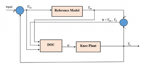
The block diagram of the overall proposed system configuration is depicted in Figure 1. The DOC's inputs include the reference model input Um, the reference model output Ym, and error feedback e. Due to the inherent second-order nature of the given system, it is suggested that the reference model be described using the standard second-order transfer function, as shown in Eq. (20) The error feedback is computed as the difference between the output of the reference model Ym and the desired output set point Yo. The value of X is computed by linearly combining these signals using adaptive gains Ke, Ky, and Ku, as shown in Eq. (21) Figure 2 depicts the intended optimal controller structure.
$\mathrm{H}(\mathrm{s})=\frac{\omega_n^2}{s^2+2 \zeta \omega_n s+\omega_n{ }^2}$ (20)
$\mathrm{X}=\left(Y_m \times K_e\right)+\left(\mathrm{e} \times K_y\right)+\left(U_m \times K_u\right)$ (21)
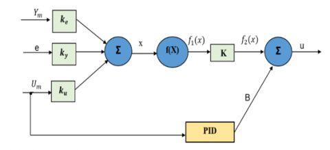
Figure 3 depicts the desired optimal controller, consisting of an MLFNN comprised of three layers and the tuned PID controller. The input variable x is utilized by the hyperbolic tangent function f(x), which exhibits a nonlinear relationship, as shown in Eq. (22) The introduced control algorithm has significant advantages over auto-tuning neural network-based controllers developed previously. These benefits include a reduction in computation time, a simplification of the structure, and an increase in control robustness [31].
$f(x)=\frac{\left(1-e^{-x}\right)}{\left(1+e^{-x}\right)}$ (22)
Figure 2. The block diagram of the proposed system configuration
Figure 3. The structure of the desired optimal controller (DOC)
The values of K and B (i.e., the PID controller's output) are used as bias weights for the input and hidden layers, respectively. Initial PID values are selected to achieve a satisfactory system response. Then the cetacean optimization algorithm is then used to fine-tune the PID gains (kp, ki, and kd) to improve the system's response further. The activation function's output, denoted f1(x) is combined with the parameter k to yield f2(x), as shown in Eq. (23). The MLFNN network is trained using the fast learning-backpropagation (FLBP) algorithm to reduce the deviation between the intended set point of the output and the actual output of the knee plant. The control signal u applied to the knee joint is explained by Eq. (24).
$f_2(\mathrm{x})=f_1(\mathrm{x}) \times \mathrm{K}$ (23)
$\mathrm{u}=\mathrm{f}_2(\mathrm{x})+\mathrm{B}$ (24)
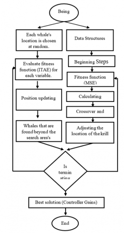
Figure 3 illustrates the detailed hybrid strategy employed to address the limitations of the current WOA. To overcome the tendency of WOA to favor local optima over global optima, a novel combined approach called WOA- KHA is proposed. The goal is to enhance the WOA's global search capability, stability, and convergence speed. KHA utilizes the mean square error (MSE) theory as a fitness function in Eq. (25), aiming to minimize the error and obtain optimal values for tuning controller parameters can be a powerful approach to optimize the performance of control systems [32]. This approach is depicted in the accompanying Figure 4.
MSE $=\frac{1}{2} \sum_{n=1}^{p o p}(\text { reference }- \text { output })^2$ (25)
Figure 4. Flowchart of combining WOA-KHO algorithm
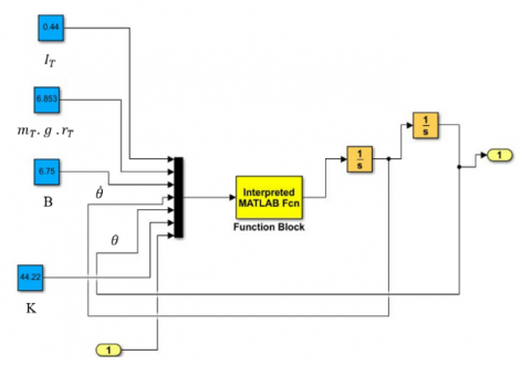
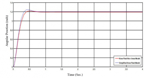
Figure 5 depicts the Simulink model of the human-robotic knee plant as described by Eq. (2) and using the parameter values described in the preceding section. Figure 6 explains the unit step response of the open loop system for the nonlinear model as specified in Figure 5 that employs Eq. (1) which includes the nonlinear parameters of the Knee joint plant dynamic model as listed in Table 1 and for the simplified model as denoted in Eq. (4) that represent the second order knee joint plant model. Based on the step response characteristics, the two responses reveal a steady-state error (es.s) of 0.19 and 0.2 for the nonlinear and simplified models, respectively, indicate that the system is slightly underdamped. For the nonlinear model, the unit step response of the closed-loop robotic human knee system is shown in Figure 7. Observations from this figure highlight certain characteristics of the closed-loop response. Notably, it shows a relatively high es.s of 0.493, accompanied by a settling time ts of 0.545 Sec. with an error tolerance of 0.02%., and a rise time tr of 0.106 Sec. These findings imply a system response with slow behavior with overshoot.
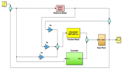
In this study, Figure 8 illustrates the Simulink model of the designed system that uses the desired DOC-based MRAC algorithm for controlling the robotic human knee. The adaptive gains ke, ky, ku are allocated the values 0.6, 0.001, and 0.001 to optimize the controller. The PID controller's parameters kp, ki, and kd are fine-tuned to accomplish enhanced system response, with specific values of 0.80, 1.29, and 0.90, respectively. By taking ζ=1 and ωn=10 and substituting these values in Eq. 20, the transfer function of the reference model is explained in Eq. (26).
$\mathrm{TF}(\mathrm{s})=\frac{100}{s^2+20 s+100}$ (26)
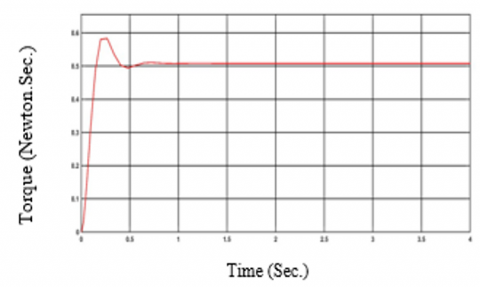
Figure 9 explains the response of the proposed controller. This figure demonstrates that the controller's response stabilizes at torque =50.97 (Newton. Sec.). This value is well within the accepted range of control signals, making it the optimal controller for the investigation's robotic human leg plant.
Figure 5. Simulink model of the robotic human knee plant
Figure 6. The unit step response of the open loop system robotic human knee for nonlinear and simplified models
Figure 7. The unit step response of the closed loop for the robotic human knee system
Figure 10 depicts the unit-step response of the robotic human knee system using the proposed DOC-based MRAC algorithm. Implementing the proposed controller enhances system response and eliminates es.s, resulting in a es.s of zero. However, the system's ts=2.52 Sec. at an error tolerance of 0.02%, indicating a relatively slow response due to the nonlinearity of the dynamic knee joint model as specified in Eq. (1), and a rise time tr=1.602 Sec.
Figure 8. Simulink model of the system using the desired DOC-based MRAC algorithm for the robotic human knee
Figure 9. The response of the desired DOC-based MRAC controller
Figure 10. The unit step response of the system using the desired DOC-based MRAC algorithm for the robotic human knee
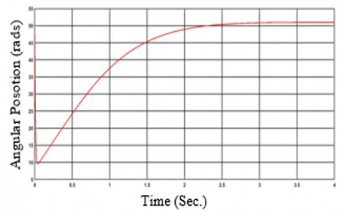
To enhance the system's performance and achieve optimal response, an optimization technique is introduced to reduce the system's settling time ts and accelerate its overall response. Figure 11 depicts the unit step response of the robotic human knee system using the proposed DOC-based MRAC algorithm optimized with GA. The simulation results demonstrate a not significant improvement in the system's performance when the GA is employed to tune the parameters of the proposed controller. The optimization technique implemented through GA effectively reduces the system's settling time ts to 0.56 Sec. with an error tolerance of 0.02%. Simultaneously, it maintains a rise time tr of 0.45 Sec. and a small acceleration in the overall response. Yet, a steady-state error es.s of 0.1 persists.
Figure 11. The unit step response of the system using GA for tuning parameters of the desired DOC-based MRAC
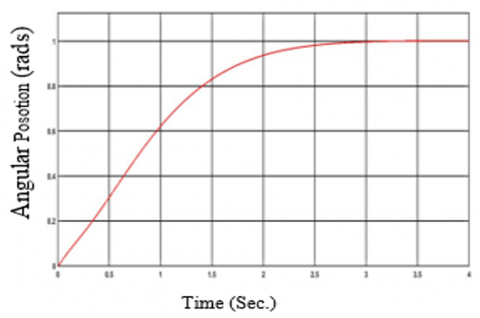
Figure 12 presents the unit step response of the robotic human knee system using the proposed DOC-based MRAC algorithm optimized with PSO, demonstrating a slight improvement in system performance. The optimization technique reduces settling time ts to 0.26 Sec. with an error tolerance of 0.02%. Simultaneously, it maintains a rise time tr of 0.15 Sec. and accelerates the overall response without minimizing steady-state error es.s.
Figure 12. The unit step response of the system using PSO for tuning parameters of the desired DOC-based MRAC
Figure 13. The unit step response of the system using WOA for tuning parameters of the desired DOC-based MRAC
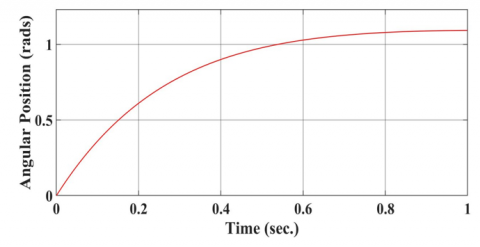
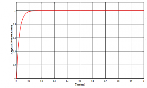
Figure 13, the unit step response of the robotic human knee system using the proposed DOC-based MRAC algorithm optimized with WOA. The simulation results demonstrate significant improvements in the system's performance when the WOA is employed to tune the parameters of the proposed controller. The optimization technique reduces settling time effectively reduces the system's settling time ts to 0.082 Sec. with an error tolerance of 0.02%. Simultaneously, it maintains a rise time tr of 0.07 Sec. and accelerates the overall response while minimizing steady-state error es.s to zero. These findings indicate the successful optimization of the controller's parameters through the WOA-based approach, leading to enhanced efficiency and precision in controlling robotic knee flexion during gait.
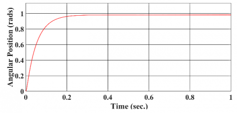
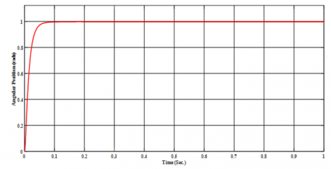
Figure 14 introduces the unit step response of the robotic human knee system utilizing the proposed DOC-based MRAC algorithm optimized with the Combined WOA and KHO, exhibiting further improvement. The joint optimization approach outperforms the use of WOA alone, achieving reduced settling time ts to 0.043 Sec. at an error tolerance of 0.02%, Simultaneously, it maintains a rise time tr of 0.029 Sec and accelerates the overall response with and zero steady-state error es.s. The synergistic effect of these nature-inspired algorithms enabled a comprehensive exploration of the parameter space, leading to the identification of an optimal parameter set for the controller.
Figure 14. The unit step response of the system using WOA-KHO for tuning parameters of the desired DOC-based MRAC
In general, the simulation outcomes unequivocally illustrate the efficacy of both the WOA-based and Combined WOA-KHO methodologies in enhancing the performance of the system. By integrating optimization techniques, the controller's parameters were refined, resulting in improved gait control and a walking experience that is more comfortable and natural for people with mobility impairments. Furthermore, further enhancements in the system's response characteristics were observed with the integration of WOA and the Combined WOA-KHO optimization approach. These improvements encompassed decreases in steady-state error, settling time, rise time, and overshoot.
The integration of KHO and WOA yields distinctive aspects that set it apart from the GA, PSO, and WOA algorithms individually. WOA draws inspiration from the foraging behavior of whales to optimize exploration in space. On the other hand, KHO uses swarm intelligence that simulates collaborative behaviors noticed in nature to enhance its capabilities of exploration.
The incorporation of the WOA-KHO approach utilizes the characteristics of both WOA and KHO to make it easier to thoroughly study and adjust the settings of the controller effectively. Consequently, the developed optimization algorithm makes it more thorough and effective, gives better control accuracy and system behavior. This optimization algorithm combines multiple algorithms to improve robot performance. It reduces errors over time, speeds up how quickly the robot becomes stable, and optimizes the time it takes to reach its peak performance. As a result, this approach makes robots more effective and responsive, making it a valuable tool for advanced robot control.
In this paper, the controller is designed to use a model of the MRAC algorithm-based DOC. For optimizing this algorithm, advanced optimization algorithms are used. The results of the simulation explain that the combination of these algorithms enhances the performance of the controller and efficiency. This gives an exception of the controller to be validated using experimental data, which will give further evidence of its accuracy.
An innovative algorithm has been introduced in this work to enhance the movements of the robotic knee during walking. This knee robotic system is improved greatly by using a combination of the DOC-based MRAC algorithm with the WOA optimization method and WOA-KHO as a combination algorithm. The results of the simulation explain that these enhancements in the control system lead to minimize errors, speed up the response of the system, and reducing overshooting with higher precision and the efficiency of the robotic knee system. This work has provided the significance of designing robotic knee prostheses utilizing optimization methods that mimic the natural systems and the control methods which are adjusted according to changing conditions.
The future expectations and consequences of these findings include methodologies of rehabilitation, offering high developments in the clinical environments. The implementation of the interventions of personalized rehabilitation, which integrate the refined strategies of the control and optimized algorithms, provides potential enhancements in mobility, the outcomes of the rehabilitation, and the quality of overall life for people with mobility impairments. The enhanced accuracy and productivity exhibited in this research indicate a potentially fruitful direction for the creation of customized and more efficacious rehabilitation approaches for people with mobility impairments. In line with the overarching goal of enhancing the general well-being of individuals with mobility impairments, this research ultimately possesses the capacity to substantially improve their walking experience.
The authors thank Mustansiriyah University (www.uomustansiriyah.edu.iq) Baghdad-Iraq for its support in the present work.
[1] Zaier, R., Dirdiry, O. (2019). Legged robots with human morphology: Design and control. 2019 International Conference on Signal, Control and Communication, SCC, pp. 302–307. https://doi.org/10.1109/SCC47175.2019.9116106
[2] Jaeger, L., De Souza Baptista, R., Basla, C., Capsi-Morales, P., Kim, Y.K., Nakajima, S., Piazza, C., Sommerhalder, M., Tonin, L., Valle, G., Riener, R., Sigrist, R. (2023). How the cybathlon competition has advanced assistive technologies. Annual Review of Control, Robotics, and Autonomous Systems, 6: 447-476. https://doi.org/10.1146/ANNUREV-CONTROL-071822-095355
[3] Baud, R., Manzoori, A.R., Ijspeert, A., Bouri, M. (2021). Review of control strategies for lower-limb exoskeletons to assist gait. Journal of Neuro Engineering and Rehabilitation, 18: 1-34. https://doi.org/10.1186/S12984-021-00906-3
[4] Driessen, J.J.M., Laffranchi, M., De Michieli, L. (2023). A reduced-order closed-loop hybrid dynamic model for design and development of lower limb prostheses. Wearable Technologies, 4: e10. https://doi.org/10.1017/WTC.2023.6
[5] Sun, Y., Tang, H., Tang, Y., Zheng, J., Dong, D., Chen, X., Liu, F., Bai, L., Ge, W., Xin, L., Pu, H., Peng, Y., Luo, J. (2021). Review of recent progress in robotic knee prosthesis related techniques: Structure. Actuation and Control. Journal of Bionic Engineering, 18(4): 764-785. https://doi.org/10.1007/S42235-021-0065-4/METRICS
[6] Wu, A.R. (2021). Human biomechanics perspective on robotics for gait assistance: Challenges and potential solutions. Proceedings of the Royal Society B, 288(1956): 20211197. https://doi.org/10.1098/RSPB.2021.1197
[7] Rifaï, H., Mohammed, S., Daachi, B., Amirat, Y. (2012). Adaptive control of a human-driven knee joint orthosis. 2012 IEEE International Conference on Robotics and Automation, pp. 2486–2491. https://doi.org/10.1109/ICRA.2012.6225064
[8] Chevalier, A., Ionescu, C.M., De Keyser, R. (2014). Model-based vs auto-tuning design of PID controller for knee flexion during gait. In 2014 IEEE International Conference on Systems, Man, and Cybernetics (SMC), pp. 3878-3883. https://doi.org/10.1109/SMC.2014.6974536
[9] Bkekri, R., Benamor, A., Alouane, M.A., Fried, G., Messaoud, H. (2018). Robust adaptive sliding mode control for a human-driven knee joint orthosis. Industrial Robot: An International Journal, 45(3): 379-389. https://doi.org/10.1108/IR-11-2017-0205
[10] Kohli, C., Neha, K., Chandar, T.S. (2017). Design of UDE based robust tracking controller for knee-joint orthosis. 2017 IEEE International Conference on Industrial and Information Systems (ICIIS), pp. 1–6. https://doi.org/10.1109/ICIINFS.2017.8300350
[11] Khalaf, P., Warner, H., Hardin, E., Richter, H., Simon, D. (2018). Development and experimental validation of an energy regenerative prosthetic knee controller and prototype. In Dynamic Systems and Control Conference 51890: V001T07A008. https://doi.org/10.1115/DSCC2018-9091
[12] Liang, X., Xu, S., Liu, Y., Sun, L. (2022). A modified whale optimization algorithm and its application in seismic inversion problem. Mobile Information Systems, 2022: 1-18. https://doi.org/10.1155/2022/9159130
[13] Karam, E.H., Abdul-Jaleel, N.S., Salah, B.J. (2020). Design of hybrid Neuro-Robust deadbeat controller for higher order linear systems based on optimized mixed reduction method. International Review of Applied Sciences and Engineering, 11(3): 251-260. https://doi.org/10.1556/1848.2020.00090
[14] Venter, G., Sobieszczanski-Sobieski, J. (2012). Particle swarm optimization. AIAA Journal, 41: 1583–1589. https://doi.org/10.2514/2.2111
[15] Karaboga, D., Basturk, B. (2007). A powerful and efficient algorithm for numerical function optimization: Artificial bee colony (ABC) algorithm. Journal of global optimization, 39: 459-471. https://doi.org/10.1007/s10898-007-9149-x
[16] Dorigo, M., Birattari, M., Stutzle, T. (2006). Ant colony optimization. IEEE Computational Intelligence Magazine, 1(4): 28-39. https://doi.org/10.1109/MCI.2006.329691
[17] Wu, H.S., Zhang, F.M. (2014). Wolf pack algorithm for unconstrained global optimization. Mathematical Problems in Engineering, 2014: 465082. https://doi.org/10.1155/2014/465082
[18] Gandomi, A.H., Alavi, A.H. (2012). Krill herd: A new bio-inspired optimization algorithm. Communications in Nonlinear Science and Numerical Simulation, 17(12): 4831-4845. https://doi.org/10.1016/J.CNSNS.2012.05.010
[19] Ma, L., Cheng, S., Shi, Y. (2020). Enhancing learning efficiency of brain storm optimization via orthogonal learning design. IEEE Transactions on Systems, Man, and Cybernetics: Systems, 51(11): 6723-6742. https://doi.org/10.1109/TSMC.2020.2963943
[20] Mirjalili, S., Lewis, A. (2016). The whale optimization algorithm. Advances in Engineering Software, 95: 51-67. https://doi.org/10.1016/j.advengsoft.2016.01.008
[21] Liang, X., Zhang, Z. (2022). A whale optimization algorithm with convergence and exploitability enhancement and its application. Mathematical Problems in Engineering, 2022: 2904625. https://doi.org/10.1155/2022/2904625
[22] Jensi, R., Jiji, G.W. (2016). An improved krill herd algorithm with global exploration capability for solving numerical function optimization problems and its application to data clustering. Applied Soft Computing, 46: 230-245. https://doi.org/10.1016/J.ASOC.2016.04.026
[23] Aloui, M., Hamidi, F., Jerbi, H., Omri, M., Popescu, D., Abbassi, R. (2021). A chaotic krill herd optimization algorithm for global numerical estimation of the attraction domain for nonlinear systems. Mathematics, 9(15): 1743. https://doi.org/10.3390/MATH9151743
[24] Ghith, E.S., Tolba, F.A.A. (2022). Real-time implementation of tuning PID controller based on whale optimization algorithm for micro-robotics system. In 2022 14th International Conference on Computer and Automation Engineering (ICCAE), pp. 103-109. https://doi.org/10.1109/ICCAE55086.2022.9762448
[25] Hu, Z., Norouzi, H., Jiang, M., Dadfar, S., Kashiwagi, T. (2022). Novel hybrid modified krill herd algorithm and fuzzy controller based MPPT to optimally tune the member functions for PV system in the three-phase grid-connected mode. ISA Transactions, 129: 214-229. https://doi.org/10.1016/J.ISATRA.2022.02.009
[26] Yu, L., Xie, L., Liu, C., Yu, S., Guo, Y., Yang, K. (2022). Optimization of BP neural network model by chaotic krill herd algorithm. Alexandria Engineering Journal, 61(12): 9769-9777. https://doi.org/10.1016/j.aej.2022.02.033
[27] Wei, C.L., Wang, G.G. (2020). Hybrid annealing krill herd and quantum-behaved particle swarm optimization. Mathematics, 8(9): 1403. https://doi.org/10.3390/MATH8091403
[28] Zhang, Z., Ding, S., Sun, Y. (2020). A support vector regression model hybridized with chaotic krill herd algorithm and empirical mode decomposition for regression task. Neurocomputing. 410: 185–201. https://doi.org/10.1016/J.NEUCOM.2020.05.075
[29] Mezher, L.S., Abbass, A.M., Saleh, B.J.( 2023). A Comparative study of a hybrid approach combining caesar cipher with triple pass protocol and krill herd optimization algorithm (KHO)-based hybridization. International Journal of Intelligent Engineering and Systems, 16. https://doi.org/10.22266/ijies2023.1231.15
[30] Enbiya, S., Mahieddine, F., Hossain, A. (2011). Model reference adaptive scheme for multi-drug infusion for blood pressure control. Journal of Integrative Bioinformatics, 8(3): 43-56. https://doi.org/10.1515/JIB-2011-173/MACHINEREADABLECITATION/RIS
[31] Anh, H.P.H., Nam, N.T. (2011). A new approach of the online tuning gain scheduling nonlinear PID controller using neural network. PID Control, Implementation and Tuning, 1-24. https://doi.org/10.5772/15964
[32] Saleh, B.J., Al-Aqbi, A.T.Q., Saedi, A.Y.F., Abdalhasan Salman, L. (2018). Comparative study of inspired algorithms for trajectory-following control in mobile robot. IJ Modern Education and Computer Science, 9: 1-10. https://doi.org/10.5815/ijmecs.2018.09.01