Fadwa Farchi*![]() | Badr Touzi | Chayma Farchi
| Badr Touzi | Chayma Farchi![]() | Charif Mabrouki
| Charif Mabrouki![]()
© 2024 The authors. This article is published by IIETA and is licensed under the CC BY 4.0 license (http://creativecommons.org/licenses/by/4.0/).
OPEN ACCESS
Amidst the rapid urbanization and the consequent surge in urban population on a global scale, the significance of efficient transportation systems has never been more pronounced. This is particularly true in critical sectors like humanitarian aid, healthcare, and pharmaceutical logistics, which face unique challenges and costs that deviate from the usual logistical norms. Strikingly, in Morocco, there's a notable absence of comprehensive studies on pharmaceutical transportation, particularly concerning the associated costs and delivery conditions. This glaring gap in research underscores the pressing need for the development of a tailored model that squarely addresses these issues. Pharmaceutical transportation presents a multifaceted landscape characterized by high-dimensional regression or classification challenges. It's further complicated by the intricacies of variable selection, especially when dealing with interrelated predictors. In this context, the Random Forests algorithm emerges as an appealing solution for both classification and regression tasks. It has demonstrated robust predictive performance and the capacity for variable selection through importance measures. In this comprehensive manuscript, we propose an innovative cost prediction model specifically tailored for pharmaceutical transport within Morocco. To set the stage for this model, we embark on a theoretical exploration of the significance of permutation importance within the context of additive regression models. This endeavor offers insights into how the correlation between predictors influences the importance of permutations. Building on this theoretical foundation, we proceed to establish our predictive cost scheme. Our model exhibits a commendable predictive performance, surpassing an accuracy threshold of 75%. This achievement underscores the robustness of the Random Forests algorithm in capturing the complexities of transportation. This multifaceted approach to cost prediction within the realm of pharmaceutical transportation in Morocco stands to provide valuable insights and practical solutions for this critical sector.
random forest, pharmaceutical transport, machine learning, forecasting
In the field of pharmaceutical transport, ensuring the safe and efficient delivery of pharmaceutical products is paramount. Enhancing the performance of the transportation process involves leveraging various algorithms to address different facets, including route optimization, delivery timeliness, cost reduction, and overall logistical efficiency. To determine the most effective algorithm for pharmaceutical transport, it's imperative to conduct thorough testing and evaluation.
Urban logistics grapples with persistent challenges, especially in finding a harmonious balance among cost-effectiveness, duration, and technological compatibility. Scientific literature has underscored the pivotal role of Artificial Intelligence (AI) in tackling these urban logistics challenges. Several studies have highlighted the advantages of AI, Including the utilization of the Ground Penetrating Radar (GPR) for monitoring road transport framework [1], forecasting energy transport and CO2 emissions [2], and the utilization of emerging technologies like geo-information, data analysis, and machine learning for enhancing smart city transport [3]. The implementation of machine learning (ML) and deep learning (DL) methods and strategies has significantly contributed to predictive modeling, planning, and uncertainty analysis in urban development [4]. However, while traditional models play a crucial role in managing transportation flows across various industries, there's a dearth of specific publications focused on pharmaceutical or medical transport.
Pharmaceutical distribution and transportation play a pivotal role in the pharmaceutical industry, particularly in regions characterized by numerous hospitals and pharmacies that receive multiple daily deliveries from local warehouses and wholesale distributors [5]. Morocco, boasting an impressive 12,000 pharmacies and a combination of 613 private and 155 public hospitals, presents a fertile ground for research within the pharmaceutical sector.
Pharmaceutical distribution is a multifaceted subject that demands meticulous analysis and monitoring. It necessitates control over various parameters to effectively manage transportation costs, encompassing factors such as departure and arrival coordinates, tire pressure, transport temperatures, freight weight, fuel consumption, and CO2 emissions. These parameters exert a significant influence on the total cost of transport, with CO2 emissions showing a strong correlation with it. Recognizing the considerable contribution of vehicles used in pharmaceutical logistics to air pollution in urban areas [6], there is a compelling need to study and mitigate CO2 emissions stemming from these vehicles.
The literature presents numerous experiments conducted in various cities, identifying key areas for enhancement in the urban distribution of pharmaceutical products. These areas include reductions in lead time, CO2 emissions, transport expenses, the number of vehicles involved, and the daily frequency of trips [7].
In concrete terms, non-sustainability generates a monetary penalty for companies. As long as the measurement of CO2 emissions or fossil fuel consumption turns out to be large or significant, the cost of transport itself becomes more expensive.
In this paper, we introduce a model for predicting the cost of urban pharmaceutical transport. Focusing exclusively on the urban transport of pharmaceutical products is driven by the unique logistical challenges posed by urban environments. The density of population, traffic congestion, stringent regulations, and specific environmental conditions in urban areas significantly impact the costs and logistics of pharmaceutical transportation. This targeted approach allows for a more precise analysis of relevant variables, providing accurate insights and tailored recommendations to address the distinctive logistics challenges inherent to urban settings.
Several methods were considered, with Random Forests—known for their superior performance—being retained for its ability to rectify decision trees' propensity to overfit their training data. Additionally, we outline the data collection and processing procedures, which play a pivotal role in our approach. Correlation and feature importance studies are emphasized, particularly concerning the algorithm employed to enhance the model.
Artificial intelligence has made significant inroads into both the pharmaceutical and distribution domains, which are sometimes merged under the purview of the Internet of Things (IoT) [8]. These are key areas of focus in our research framework. Machine learning-based models for predicting transportation costs are gaining prominence in the literature. In our case, the cost is a complex dependent variable linked to multiple inputs and constraints. Well-designed and articulated models have the potential to guide decision-making processes related to pharmaceutical product transportation. They allow providers to anticipate the inputs or factors that need to be addressed for effective budgetary management [9].
In the upcoming steps, we will initiate the process by carefully selecting treatment variables, dedicating time to collect and preprocess them in terms of importance and correlation as a sorting mechanism. Subsequently, we will choose a set of artificial intelligence-based cost prediction methods. These methods will undergo rigorous evaluation based on criteria such as error rates and precision, allowing us to identify the most robust predictive model. This meticulous approach ensures that our final selection aligns with the specific requirements of accuracy and reliability for predicting transportation costs in the context of our study.
2.1 Literature search
In the pharmaceutical sales sector, effective value chain and logistics management are indispensable. Transportation and storage expenses frequently constitute a substantial portion, often exceeding 40%, of the overall logistics cost. In response to this challenge, a variety of solutions have been explored. As outlined, technologies such as RFID (radio frequency identification), IoT (Internet of Things), and blockchain have been integrated into these systems to facilitate traceability [10], data storage, and processing [11]. These advanced technologies hold significant promise in improving the efficiency and transparency of pharmaceutical logistics processes.
RFID technology involves the use of wireless communication to identify and track objects equipped with RFID tags. In pharmaceutical transportation, RFID plays a pivotal role in enhancing traceability and visibility throughout the supply chain. Each pharmaceutical product can be assigned a unique RFID tag, allowing real-time monitoring of its location, condition, and transit history. This not only reduces the risk of counterfeiting but also enables precise tracking, ensuring the integrity of sensitive pharmaceuticals during transportation.
On the other hand, the Internet of Things (IoT) involves the interconnectivity of appliances and systems, enabling them to collect and exchange data. In pharmaceutical transportation, IoT facilitates the integration of various sensors and devices, creating a smart and responsive supply chain. Temperature-sensitive pharmaceuticals, for example, can be monitored in real-time using IoT sensors to ensure that they remain within specified temperature ranges during transit. This level of visibility is crucial to maintaining the efficacy of pharmaceutical products and complying with stringent regulatory requirements.
The synergy between RFID and IoT in pharmaceutical transportation enhances overall supply chain efficiency and integrity. RFID technology provides unique identifiers, while IoT sensors gather real-time data on environmental conditions, allowing for a comprehensive view of the entire transportation process. This not only mitigates the risk of product spoilage or damage but also enables proactive decision-making to address potential issues before they escalate.
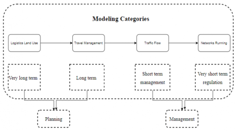
While examining pharmaceutical logistics from a broader standpoint, it falls within the realm of standard logistics. In this context, four fundamental categories of existing models are discernible. However, none of these models are specifically designed for predicting urban transportation costs concerning pharmaceutical products. As a result, our research is geared towards addressing travel planning and route management, critical components within urban logistics [5]. This model, although explored by various researchers, remains a work in progress. The notable advantage, in contrast to land-based solutions, is that while the spatial scales are global, the costs associated with implementing travel demand solutions are relatively manageable [12, 13]. For a visual representation, refer to Figure 1.
Figure 1. Modeling categories
The forecasting model we developed was designed to cater to travel management within the pharmaceutical sector, with a specific emphasis on transporting pharmaceutical goods. These goods include products sourced from pharmaceutical laboratories or biotechnology companies.
We selected this particular area of application due to the delicate nature of the transported products, which can be easily damaged if the transportation conditions are not met. Additionally, the pharmaceutical coefficient, which reflects the importance and sensitivity of the pharmaceutical goods, played a significant role in our choice. The transportation of pharmaceutical products bears resemblance to the transportation of perishable items, such as edible or chemical liquids, as well as the transportation of fresh and dry goods in the agri-food industry. This similarity arises from the fact that pharmaceutical goods are sensitive to temperature and other factors, leading to rapid deterioration if not properly handled. These factors differ from one scheme to another but are generally due to the long transport times, the speed of the vehicle, the pressure exerted on the boxes, or even the shocks between the products. The term “medication”, within the meaning of this law, means any substance or composition claimed to possess healing properties or preventive measures against human or animal diseases, as well as any product that may be administered to humans or animals to establish a medical diagnosis or restor, correcting or modifying their organic functions (Article L5111-1, Public Health French Code).
2.2 Categorization of transport vehicles
Various categories of products require very special handling and transportation. This is the case of dangerous goods that can harm carriers or consumers or even products that humans or other living being will consume. For safe transport of perishable foodstuffs, it is possible to use refrigerated vehicles (van, utility vehicle, truck, etc.) available in 4 types:
The isothermal vehicle: this vehicle offers an insulated body on all its surfaces to reduce heat exchange through the walls;
The refrigerated vehicle: this vehicle is equipped with a mechanical device capable of generating cold, which allows you to adjust the temperature. Ideal for transporting cold over long distances;
The refrigerated car: this isothermal car has a non-mechanical cold device offering the possibility of adjusting the temperature inside the body;
The calorific vehicle: this device raises the temperature inside the empty box and maintains it for a minimum of 12 hours.
It is important to note that this type of product is not only sensitive but is governed by laws that necessarily respond to logistical issues. Apart from incident management, good hygiene and maintenance of vehicles, the temperature is one of the major characteristics.
Refrigerated vehicles are the ones that most comply with medical transport regulations. The 2nd category is then the most suitable in our case since pharmaceutical products must be kept at a given temperature.
According to factors of geographical location (Position of application which is Morocco), the distribution of pharmaceutical products is done only utilizing transport of medium capacity. Generally, these are vehicles between a motorcycle and a valve. As Motorcycles offer a very reduced capacity which forces the driver to do much more travel, as well as the lack of security of the carrier we ignore this latter.
The chosen vehicle is a refrigerated van, with a payload of 610 Kg, useful height of 1.16 m, useful length of 1.79 m, and useful volume: of 2.70 m3 that represents the following parameters:
·Air conditioning
·Cruise control + speed limiter
·Electric Pack: electric and heated exterior mirrors, 12 V socket in the rear area, 1 folding key
·ESP (stability control) + Hill Assist
·Visibility Pack: automatic switching on of lights + automatic windscreen wipers
2.3 Site selection
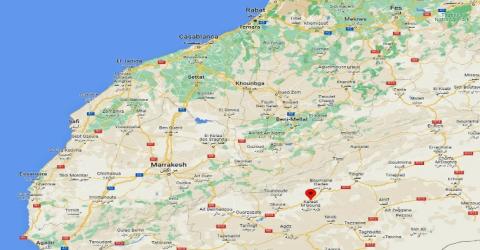
The selection of urban areas for our study was a pivotal and meticulously planned decision. Our aim was to encompass cities that authentically represent the diverse urban dynamics present throughout Morocco, extending from the northern regions to the southern territories, all while considering the intricate web of intra-industry trade connections. In Figure 2, we've highlighted our choice of seven cities, each serving as a faithful reflection of the urban landscapes in Morocco. These cities have been carefully chosen to reflect the realistic transportation patterns within pharmaceutical distribution.
Figure 2. Map
To enhance the accuracy and authenticity of our research, we've incorporated real driver routes from pharmaceutical product distribution, creating a scenario where some routes are frequently repeated while others appear only once in our observations. This aspect is crucial, as it aligns our model with the intricacies of these routes and ensures the recognition of both repetitive and non-repetitive pathways.
Our selected cities, which include Casablanca, Rabat, Essaouira, Fes, Marrakech, El Jadida, and Safi, hold the status of tourist destinations. Consequently, they experience substantial traffic congestion and jams, driven by the considerable demand for pharmaceutical products. To provide a more visual representation of these chosen cities, we've included a satellite view in the image below, allowing a closer look at the urban landscapes where our data collection took place.
Our chosen sector of focus pertains to the intricate domain of pharmaceutical product transportation within the cities mentioned earlier. In this extensive operational landscape, these pharmaceutical goods embark on a journey originating from the manufacturers' storage facilities. Their ultimate destinations are widespread and encompass a multitude of crucial institutions, including but not limited to pharmacies, hospitals, clinics, as well as popular shopping hubs and supermarkets. This comprehensive distribution network ensures that pharmaceutical products efficiently reach their intended recipients, catering to the diverse and dynamic needs of urban communities.
2.4 Approach description
Our approach is primarily centered on the development of a model designed to predict the transportation costs associated with pharmaceutical products, our designated "target." Our initial steps involved the meticulous selection of parameters and inputs, guided by a comprehensive correlation study. This in-depth analysis aimed to understand the significance and influence of various inputs on the ultimate cost, the output. Before finalizing our model, we embarked on a comparative exploration of different algorithms, employing diverse mathematical techniques to evaluate their performance. This evaluation relied on measuring the deviations between actual values and the model's estimations, as well as assessing precision.
Our contribution to this domain unfolds as a two-model program: it encompasses a semantic model and a predictive model, as previously outlined.
The choice of vehicle for pharmaceutical product transportation is anchored in two fundamental realities: adherence to Morocco's regulations concerning refrigerated vehicles and the typical freight quantities, which are moderate in comparison to other countries. This selection significantly impacts our model as it directly influences payload capacity, fuel consumption, carbon emissions, and several other critical factors.
3.1 Random forest algorithm
Random Forest is a potent machine-learning algorithm utilized for tasks involving both classification and regression. This method belongs to the category of ensemble learning, where predictions are generated by aggregating outputs from numerous decision trees. This collaborative approach enhances the accuracy and robustness of predictions. Let's delve into how Random Forest operates:
Decision Trees: Random Forest begins with a collection of decision trees. A decision tree is a flowchart-like structure that recursively splits the dataset into smaller subsets. Each split is based on a feature's value, and the goal is to create "leaves" at the bottom of the tree that contain data points with similar characteristics.
Bootstrapping plays a crucial role in the Random Forest algorithm. In the construction of each tree within the ensemble, a random subset of the original data is chosen through a technique known as bootstrapping. This process entails the random selection of data points from the original dataset, allowing for replacement. Consequently, some data points may be sampled multiple times, while others may not be included at all in the creation of a specific tree. This methodology contributes to the diversity and robustness of the Random Forest by exposing each tree to slightly different variations of the training data.
Feature Selection in Random Forest is a critical aspect of its functioning. In the process of constructing each decision tree, a random subset of features is taken into account at each node for the split. This deliberate introduction of randomness serves to decorrelate the individual trees within the ensemble. The purpose is to prevent any single powerful feature from exerting undue influence over the entire model. This strategy contributes to the diversity of the trees, promoting a more robust and generalized predictive performance.
Growing Trees: The decision trees are grown deep, meaning they're allowed to have many levels and make complex splits. This might lead to overfitting for individual trees, but that's okay because the ensemble approach will help mitigate this.
Voting (Classification) or Averaging (Regression): When it's time to make predictions, each tree in the forest "votes" (in classification) or provides an output (in regression). For classification problems, the class with the majority of votes is the predicted class. For regression, the outputs are averaged.
The strength of Random Forest lies in its ability to reduce overfitting and increase the model's generalization to new, unseen data. This is because the ensemble of diverse decision trees compensates for the shortcomings of individual trees. Additionally, Random Forest provides a measure of feature importance, which can be helpful in understanding which features have the most influence on the model's predictions. It is a versatile and widely used algorithm in machine learning, capable of handling a wide range of data types and achieving high predictive accuracy.
We first start by collecting our data from several levels [14]. The variables retained emanate from a crossing of the most used parameters which recur in a recurring way at the level of the literature more those which are essential compared to the studied context. Subsequently a data processing to eradicate distorting values, correlations and less important variables. Afterwards, tuning of the model and the adjustment of the parameters.
The random forest algorithm is a nonparametric method dealing at the same time with both classification and regression problems. It shows good performance predictive data in practice, even in a very large framework.
The Random Forest consists of numerous decision trees, each independently trained on subsets of the training dataset. Each tree generates an estimate, and the final prediction is derived from combining these results, leading to decreased variance [15].
The core concept behind bagging is to average out a significant amount of noise from approximately unbiased models, effectively diminishing variance. Trees are well-suited for bagging, given their ability to capture intricate interactions. As to reproduce results [16], and to make good use of the random forest algorithm, we have brought several helpful libraries. The first one is the RamdomForestRegressor. Schematically, it consists in calculating the average of the predictions obtained by all the estimates of the decision trees of the random forest. As well as column transformers for data preprocessing and extraction. OneHotEncoder for encoding binary variables also that do not have a quantitative aspect. Then, the implementation of the imputation of missing data.
3.2 Implementation in our research
The use of the Random Forest method in conjunction with artificial intelligence in our study represents an innovative approach to predict transportation costs. This method relies on a rich and comprehensive database, encompassing a multitude of essential variables. Among these data points, we find information on consumption, congestion factors, travel duration, vehicle speed, route length, and even customer satisfaction indicators. The ingenuity of this approach lies in its ability to assimilate all of these complex data points to establish subtle correlations and reveal significant trends.
When these data elements are ingested by our machine learning model based on Random Forest, a true computational alchemy takes place. The model can harness this wealth of information to accurately predict transportation costs. This prediction proves to be a valuable tool for urban logistics companies. It significantly enhances route planning, optimizes fuel consumption, and meets the evolving needs of customers. Furthermore, it contributes to more efficient cost management.
Thus, through this innovative approach, our study paves the way for substantial optimization of transportation operations, which, while economically sustainable, also addresses the current challenges of urban logistics.
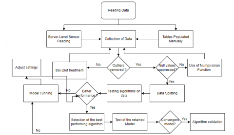
When it comes to outlining our model, we will represent it graphically, as depicted in Figure 3 below:
Figure 3. Program description
We initiate a preprocessing stage that involves bundling both numerical and categorical data.
Eq. (1) represents the diagram shown in Figure 4. which briefly represents the 2 pillars that make up our random forest program:
Random forest $=$ Tree Bagging + Features Simpling (1)
Figure 4. Random forest explanation
4.1 Entries: Variables and constraints
Persistent urban transportation challenges in Moroccan cities, as seen in many other urban areas globally, encompass a range of issues including traffic congestion, air pollution, road accidents, high transportation costs, and traffic gridlocks. This paper specifically focuses on developing a model for transportation cost analysis, with a particular emphasis on accounting for unforeseen expenses.
Table 1. Designation and classification of variables
|
Types of Data |
Variables |
|
Transport data |
X5,X6,X8,X9,X10,X11,X12,X14X16,X20,X21 |
|
Company structure data |
X1,X2,X3,X4 |
|
Environment and data |
X19,X22,X23,X24,X25 |
|
Business sector data |
X7,X13,X15,X17 |
|
Durability data |
X18,X26 |
|
Variables |
Designations |
|
X1 |
Vehicle per fleet |
|
X2 |
Fleet Number |
|
X3 |
Driver ID |
|
X4 |
Trip ID |
|
X5 |
Departure coordinates |
|
X6 |
Arrival coordinates |
|
X7 |
Delta T -Min |
|
X8 |
Distance - Km |
|
{X9, X10, X11, X12} |
Tire Pressure Xi / I from 9 to 12 |
|
X13 |
Temperature |
|
X14 |
Weight Freight |
|
X15 |
Delta T-H |
|
X16 |
Speed – Km/H |
|
X17 |
Consumption per trip -L |
|
X18 |
Emission Co2 -kg |
|
X19 |
Number of stops per trip |
|
X20 |
Level of Service |
|
X21 |
Unforeseen delays |
|
X22 |
Number of vehicles |
|
X23 |
Concentration |
|
X24 |
Flow speed |
|
X25 |
Rate of flow |
|
X26 |
Fossil energy consumption per Ton of freight |
Once the specific field of application and transportation mode were chosen, the subsequent step involved data consolidation. The data utilized in this study was gathered over an uninterrupted 8-week duration. It is derived from real-world sources, this encompasses statistics supplied by drivers and handlers engaged in distribution, information from vehicle dashboards, GPS devices, assorted detectors and sensors, along with estimated calculations pertinent to the transportation environment. Additionally, some data points are associated with clients involved in the transportation process. Further details will be expounded below.
Data varies from one city to another. In the context of 7 cities depicted on a diagram, the routing to intermediate customers varies in four distinct ways. In some cities, distributors adhere to a fixed distribution schedule over a 9-day calendar period. In another scenario, each driver consistently serves the same destinations, with each driver assigned no more than three fixed delivery points, a practice often designed to meet customer preferences. Thirdly, some cities follow a typical demand-driven distribution approach. It's crucial to emphasize that these distribution variations primarily consider the shortest path algorithm as the initial calculation, which drivers subsequently follow. When addressing urban road transport, multiple variables can come into play. Specific criteria were established for their selection, ensuring that only relevant data was integrated. The data utilized in the analysis was diverse, coming from various sources and falling under five distinct categories as depicted in Table 1.
4.2 Variable explained: Cost per trip
Prior to defining the model's outcome, it's essential to reiterate the model's primary objective, which is forecasting. This predictive capability aims to streamline the decision-making process, empowering operators to proactively influence a critical factor with a direct impact on the model's output. In the context of pharmaceutical product transportation, the scope of this process extends to encompass risk management associated with distribution, the vulnerability of their transit, and the financial aspects of various transport-related operations [17].
We have opted to use the total transportation costs as the primary output of our program. These costs are calculated based on various factors, including consumption, delays, and handling expenses.
Predicting the cost of delivery in pharmaceutical transport serves several critical purposes:
Cost Efficiency: By accurately predicting delivery costs, pharmaceutical companies can optimize their budgets and resources, leading to cost savings in the long run.
Budget Planning: Accurate cost predictions help in budget planning and the allocation of financial resources to maintain financial stability and ensure that there are no unexpected financial burdens.
Pricing Strategies: Pharmaceutical companies can use cost predictions to set competitive pricing for their products. This is particularly important in markets with tight profit margins, where slight variations in delivery costs can impact pricing decisions.
Resource Allocation: Knowing the expected delivery costs enables companies to allocate resources efficiently. For instance, they can decide on the number of vehicles, drivers, and routes required for deliveries, reducing wastage and enhancing productivity.
Customer Service: With accurate cost predictions, companies can enhance their customer service. They can provide more reliable delivery estimates to customers.
Risk Mitigation: Predicting delivery costs allows companies to identify potential issues and uncertainties in the transportation process, mitigating the risks associated with unforeseen cost overruns.
Competitive Advantage: Companies that can accurately predict delivery costs have a competitive advantage in the market.
This constitutes a cost prediction problem involving a subset of variables, determined through the analysis of correlation and feature importance. The listed explanatory variables will be refined based on the model's findings.
4.3 Sustainability and data preparation
Emphasizing the importance of sustainability in transportation cost prediction underscores the need to integrate the costs associated with various sustainable components, denoted as X26 and X18. By incorporating these sustainability factors into the predictive model, we not only enhance the accuracy of transportation cost estimations but also contribute to a more comprehensive understanding of the environmental and social impacts associated with the transportation process. In this context, optimizing for sustainability becomes synonymous with optimizing for cost efficiency. An intriguing aspect lies in the ability to identify cost-saving measures through inverse actions on factors that traditionally escalate transportation costs. This approach aligns with the contemporary emphasis on green logistics and corporate social responsibility, where organizations are not only focused on economic efficiency but are also driven by a commitment to minimizing environmental footprints and fostering sustainable practices throughout the supply chain. Thus, the integration of sustainable components into transportation cost prediction models represents a forward-thinking strategy that not only improves economic outcomes but also aligns businesses with the imperative for responsible and eco-conscious practices.
Collecting pertinent variables from structured sources involves utilizing databases and specialized collection interfaces. Additionally, external sensor-derived datasets are taken into account, encompassing transport characteristics such as speed, temperature, and congestion estimates. After collecting the data, it is important to process the table of observations so as not to distort the model. The volume of data we have is very large. We will have to rely on cleaning to optimize our data management process.
We resort to this technique whenever we think the model may give erroneous performance if the data is implemented abruptly. Basic training data (from the primary test of the program) should be large to a certain extent with different tendencies so that the model is not bounded. In a table we gather the data of different dimensions and units of measurement. We aggregate the data by date, and we progressively feed the entries according to the selected variables. We closely explore the distribution of the latter to display the maximums, the minimums and the averages. Which, despite our prior intentions to start a selective study, confirms the need for data filtration
4.4 Outliers removal
An outlier refers to a data point or object that significantly differs from the rest of the objects, often referred to as normals. Such deviations can result from errors in measurement or execution. The process of identifying outliers is termed outlier extraction. Various methods, including visualization and mathematical formulas, can be employed for outlier detection. The elimination process is akin to removing a data item from a grouped Excel table. Visualization, particularly through boxplots, remains a crucial technique. Boxplots succinctly summarize data by representing the 25th, 50th, and 75th percentiles, providing an efficient summary of the dataset, as depicted in Figure 5. We can conveniently obtain essential information such as quartiles, median, and outliers. The model provides us with an outlier index, which is essentially a list of values that should be excluded from the dataset. These values not only provide inaccurate representations of the dataset but can also distort the predictive model.
To eliminate these outliers, we need to follow a process that involves identifying their precise positions within the dataset. This is because the various outlier detection methods yield a final result that consists of a list of data items meeting the outlier criteria based on the specific method employed.
Figure 5. Outliers’ removal
4.5 Removal of missing, absent or null values
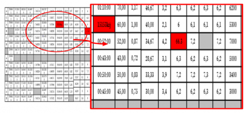
NAN serves as a constant signifying the illegitimacy of a given value, representing "Not a Number." It's important to distinguish between NAN and NULL, with NULL denoting non-existent and empty values. In our Python analysis, we identified and eliminated all null and unauthorized values. The isnan() function from the math library is employed to detect nan constants in float objects, returning True for each encountered value. Additionally, the numpy.isnan() function extends this capability to various collections like lists and arrays, generating an array with True values where nan constants are present. The removal process, illustrated in Figure 6 (extracted from our data), involved eliminating all gray and red boxes.
This figure shows the outliers that have been removed from the template. We zoom in to see closely the erroneous values that the system does not take into account, for example in red we display 2 errors: The first value is not part of the data range, while the second is entered falsely. In gray we display the empty NA boxes for missing data.
Outliers can significantly distort the accuracy and reliability of the results. These anomalies, often extreme values that deviate significantly from the typical data distribution, exert disproportionate influence on the model parameters. In the context of predicting transportation costs, outliers might represent exceptional events such as unusually high fuel prices, extreme weather conditions, or unforeseen disruptions in the supply chain. When incorporated into the training data, these outliers can skew the model's understanding of the normal patterns and lead to a biased prediction. Addressing outliers is crucial to ensure that the model generalizes well to regular scenarios and is not overly influenced by exceptional events, ultimately enhancing the model's predictive performance in real-world applications.
Figure 6. Data cleansing
Once the data is thoroughly cleansed, the next step involves constructing the model using the input variables and constraints. However, in a high-dimensional learning scenario, not all explanatory variables may be essential for predicting the variable of interest. The process of decreasing the number of explanatory variables provides a twofold benefit. Firstly, a model with fewer variables is easier to interpret. Secondly, eliminating non-informative variables helps lower prediction errors.
We undertake two reduction approaches, beginning with a correlation study between variables and identifying key features to retain only the variables that directly influence the program.
The decision to test three algorithms—Random Forest, Support Vector Machine (SVM), and Neural Network—derives from the need to explore diverse approaches in predicting pharmaceutical transportation costs. Each algorithm brings unique strengths to the table: Random Forest excels in handling complex datasets and variable importance assessment, SVM is effective in high-dimensional spaces and classification tasks, while Neural Networks demonstrate prowess in capturing intricate patterns. By evaluating these algorithms on a substantial dataset, we aim to ensure the robustness and generalizability of the chosen model. Large datasets offer a comprehensive representation of real-world scenarios, allowing for a thorough examination of algorithm performance under diverse conditions and enhancing the reliability of the final predictive model.
5.1 Correlation study- Semantic model
The correlation coefficient, often denoted as 'r' in correlation analysis, is a precise metric used to quantify the degree of linear association between two variables. It calculates this relationship by comparing the deviation of each data point from the variable's mean and using this information to indicate the degree to which the variables conform to an imaginary line drawn through the data. Essentially, correlations focus on linear connections between two variables.
It's important to note that correlation analysis exclusively considers the relationship between two variables and doesn't provide insights into more complex relationships involving multiple data points. This analysis is also unable to identify and can be influenced by the presence of outliers in the data. This underscores the significance of the outlier treatment we conducted during the initial data collection and preparation phase.
While our primary purpose is to illustrate correlations with the dependent variable, we also present the entire correlation matrix, which aggregates the most significant correlations within the system.
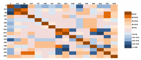
In Figure 7, we illustrate the correlation of the used variables.
Figure 7. Correlations
The color code used is simple. For a correlation ‘r’ that goes from [-1;1] we represent in bluish colors the negative correlations and in brownish the positive ones. Positivity is recognized when an increase in one variable causes an expansion in another. When the evolution of a variable is explained by the decrease of another it is a negative link. As long as we are interested in the explained variable "Total Cost", we note among the most important correlations: Distance - Km, Delta T – Min, Temperature, Tire Pressure 2, Flow speed, Number of vehicles, Unforeseen delays, Speed – Km/H, Fossil energy consumption per Ton of freight.
5.2 Features importance
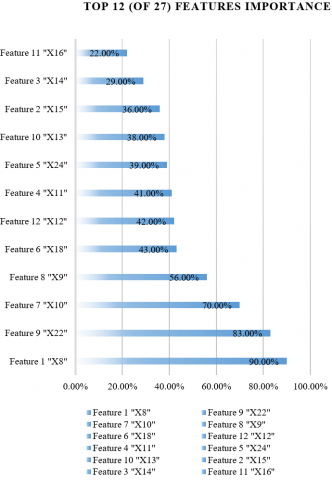
For linear models and many other model types, there exist techniques for assessing the importance of explanatory variables that exploit unique aspects of each model's structure. These methods are tailored to the specific model type in use. For instance, in linear models, the normalized regression coefficient's value or its corresponding p-value can be utilized as indicators of variable importance. In the context of tree-based models, variable importance metrics may be derived from the role of specific variables in individual trees. An exemplary case is the variable importance metric based on out-of-bag data for a random forest model [18]. Additionally, alternative approaches, such as those implemented in the XgboostExplainer package for gradient boosting and the randomForestExplainer for the random forest algorithm, are available [19]. In Figure 8, we present the outcomes of employing this method in our initial dataset.
Figure 8. Features’ importance
5.3 Results- Formal model’s performance metrics
To illustrate the results of our cost prediction model, we choose the urban area of Casablanca as it is the most complex city. The precision of a machine learning classification algorithm indicates how frequently the algorithm accurately categorizes a data point. It is computed as the count of correctly predicted data points divided by the total count of data points. In more formal terms, it is the sum of true positives and true negatives divided by the sum of true positives, true negatives, false positives, and false negatives.
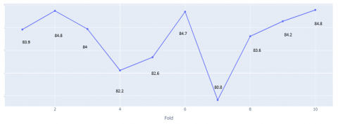
In the chosen case, the model we created manages to reach a precision interval between 80% and 84.8% for 10 folds as shown in Figure 9. This diagram represents the results of the 10 folds in terms of performance (accuracy).
Given the nature and quantity of the data, i.e. 2500 observations for 26 basic variables (with a total of approximately 67500 entries), our model had enough data for the training phase. No common calculation combination between the different variables and constraints to avoid that the model detects formulas of direct calculations of the output compared to the inputs.
Machine learning-based models can detect the curve shapes of the outputs through the trends of the inputs. Random Forest algorithm manages to break these links to make normal learning based on data only. The prediction performance is not over-adjusted.
Besides the smooth running of the learning phase of the model, the regulation of the internal parameters of the program played a very important role in the tuning phase. As it was mentioned before, we divided the data into 10 folds.
The advantage of this model is that it presents a concordance with the existing state in the literature in the field of pharmaceutical transport, and the need to predict the costs which no longer depend solely on fuel prices. For emissions of gases [6] that are harmful to human health and the planet are to be taken into account.
Customer satisfaction is quantifiable in terms of cost as well [20]. Retards and delays not taken into consideration by the carrier make the delivery cost more money.
Figure 9. 10 folds’ performance
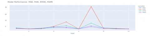
The particularity of prediction and forecasting techniques is to envisage in one way or another what should be, according to the idea that one has of reality. We collect data and then process it. This processing results in modeling in the form of equation(s) and validation. We choose the following measures as deviation/gap indicators. At this level, we also display the results of the program in terms of error in Figure 10.
Figure 10. Gap indicators – 10 folds
The mean square error (MSE for Mean Square Error or MCE for mean squared error): this is the arithmetic mean of the squared differences between model forecasts and observations. The root means square error for the worst case is 31, which can be used as a benchmark to see if the accuracy of the model improves over time.
$M S E=\frac{1}{n} \sum_{i=1}^n\left(Y_i-Y_i^{\prime}\right)^2$ (2)
The root means square error (RMSE): square root of the previous one. The weighted average error between the predictions and the actual values in this dataset is almost 5.6, which is seen that the distribution is more or less accumulated between [48:62].
$R M S E=\sqrt{M S E}=\sqrt{\frac{1}{n} \sum_{i=1}^n\left(Y_i-Y^{\prime}{ }_i\right)^2}$ (3)
The mean absolute error (EAM or MAE for Mean Absolute Error): arithmetic mean of the absolute values of the deviations. The mean of the absolute values of the errors is very low. which is in the worst case equal to 5.
$M A E=\frac{\sum_{i=1}^n\left|e_i\right|}{n}$ (4)
The Mean Absolute Percentage Error (MAPE) represents the average of absolute deviations from the observed values, expressed as a percentage. It serves as a practical indicator for comparison.
$M A P E=\frac{100 \% \sum_{t=1}^n\left|\frac{A_t-F_t}{A_t}\right|}{n}$ (5)
In this study, we've addressed a significant problem in the logistics field that has previously been identified as a research gap. We began with a literature review to pinpoint the recurring issue in the state of the art, primarily centered on calculating the total cost of urban transportation for pharmaceutical and medical products. Our contribution involves the development of a predictive model for estimating the total cost of transporting and distributing pharmaceutical and medical products, approximated using the Random Forest algorithm.
Before settling on the final algorithm (Random Forest), we constructed different models based on various algorithms, including neural networks, support vector machines, and random forests. We evaluated the performance of the Random Forest, Support Vector Machine, and Neural Networks models, which yielded accuracies of approximately 80% - 85%, 66.9% - 70%, and 61.4% - 64.3%, respectively. The Random Forest algorithm emerges as the optimal choice for predicting transportation costs when compared to Support Vector Machines (SVM) and Neural Networks. The strength of Random Forest lies in its ability to handle large datasets with numerous features, mitigate overfitting, and provide robust predictions through an ensemble of decision trees. Unlike Support Vector Machines, which might struggle with complex datasets and can be sensitive to the choice of kernel functions, and Neural Networks, which often require extensive tuning and large amounts of data, Random Forest demonstrates versatility and resilience. Its inherent capacity for feature importance assessment aids in extracting meaningful insights from the dataset, contributing to enhanced interpretability. These advantages collectively position Random Forest as a powerful and effective tool for predicting transportation costs, making it a preferred choice in data-driven decision-making scenarios.
The application of the ultimate model took place in seven different Moroccan cities as mentioned in part 2-3. Once we consolidated the data, we implemented variable selection functions and essential features. We employed five precision parameters, namely MSE, RMSE, MAE, and MAPE, to assess the degree of approximation achieved by the model. We fine-tuned the model parameters to enhance accuracy and reduce errors, ultimately achieving a prediction accuracy of about 85%. This remarkable performance can be further improved by refining the settings during the tuning phase. In contrast, algorithms such as Neural Networks and Support Vector Machines did not offer a significant accuracy boost and are better suited for tasks like traffic or red-light management, with a performance of more than 75%.
Thanks to this exceptional performance, the model can be adopted by transportation companies, particularly those involved in pharmaceutical product distribution. Managerially, the model can serve as a foundation for guiding managers and decision-makers by enabling the estimation and prediction of total transportation costs, and, if necessary, adjusting the parameters (inputs) to optimize the output.
It's worth noting that the value of this study extends beyond cost prediction; it also identifies key elements that can impact costs. We've learned that costs can be reduced by acting on specific input parameters, which in our case include factors like the distance traveled by the transport vehicle, gas consumption, temperature of goods storage, customer satisfaction, fossil energy consumption, road congestion, and traffic speed. In addition to transportation and environmental aspects of freight delivery, sustainability variables are crucial, as environmental damage can be costly, and sustainability is now a fundamental aspect of urban transportation.
Highlighting sustainability in transportation cost prediction is crucial for integrating costs related to sustainable components, denoted as X26 and X18. By incorporating these factors, our predictive model not only enhances cost estimations but also fosters a deeper understanding of environmental and social impacts in transportation. The pursuit of sustainability seamlessly aligns with cost efficiency, offering the intriguing possibility of identifying cost-saving measures by addressing factors traditionally elevating transportation costs. This approach resonates with contemporary priorities of green logistics and corporate social responsibility, showcasing a commitment to minimizing environmental footprints. Ultimately, integrating sustainable components into transportation cost prediction models reflects a forward-thinking strategy, improving economic outcomes while emphasizing responsibility and eco-conscious practices throughout the supply chain.
However, there are limitations to the results that should be acknowledged. Firstly, the model represents specific areas, and its direct applicability may require adaptation to other contexts. Secondly, the study is tailored to the Moroccan context and may not directly extrapolate to other regions without adjustments. Lastly, the distances covered in this study are limited, with a maximum of 25 km, which directly affects transportation costs, falling within a range of [10: 80] MAD per trip, with a significant concentration in the [48: 62] MAD range, as illustrated in Figure 11.
We anticipate the potential for incorporating numerous variables into the model in the future. This expansion is intended to align with possible advancements and does not undermine the credibility of our current work. Subsequent research can be built upon the foundation laid in this paper. The model can be adapted for application in various other sectors by adjusting the scopes or the context under examination. This would provide an opportunity to test the model's generality and assess its accuracy when applied across different sectors.
Figure 11. Cost distribution
[1] Rasol, M., Pais, J.C., Pérez-Gracia, V., Solla, M., Fernandes, F.M., Fontul, S., Ayala-Cabrera, D., Schmidt, F., Assadollahi, H. (2022). GPR monitoring for road transport infrastructure: A systematic review and machine learning insights. Construction and Building Materials, 324: 126686. https://doi.org/10.1016/j.conbuildmat.2022.126686
[2] Ağbulut, Ü. (2022). Forecasting of transportation-related energy demand and CO2 emissions in Turkey with different machine learning algorithms. Sustainable Production and Consumption, 29: 141-157. https://doi.org/10.1016/j.spc.2021.10.001
[3] Ang, K.L.M., Seng, J.K.P., Ngharamike, E., Ijemaru, G.K. (2022). Emerging technologies for smart cities’ transportation: Geo-information, data analytics and machine learning approaches. ISPRS International Journal of Geo-Information, 11(2): 85. https://doi.org/10.3390/ijgi11020085
[4] Woschank, M., Rauch, E., Zsifkovits, H. (2020). A review of further directions for artificial intelligence, machine learning, and deep learning in smart logistics. Sustainability, 12(9): 3760. https://doi.org/10.3390/su12093760
[5] Huff-Rousselle, M., Burnett, F. (1996). Cost containment through pharmaceutical procurement: A caribbean case study. The International Journal of Health Planning and Management, 11(2): 135–157. https://doi.org/10.1002/(sici)1099-1751(199604)11:2%3c135::aid-hpm422%3e3.0.co;2-1
[6] De Carvalho, P.P.S., Kalid, R.D.A., Moya Rodriguez, J.L. (2019). Evaluation of the city logistics performance through structural equations model. IEEE Access, 7: 121081–121094. https://doi.org/10.1109/ACCESS.2019.2934647
[7] Forkert, S., Eichhorn, C. (2008). Innovative approaches in city logistics: Inner-city night delivery. Niches.
[8] Aliahmadi, A., Nozari, H., Ghahremani-Nahr, J. (2022). Big Data IoT-based agile-lean logistic in pharmaceutical industries. International Journal of Innovation in Management, Economics and Social Sciences, 2(3): 70-81. https://doi.org/10.52547/ijimes.2.3.70
[9] Stephenson, N., Shane, E., Chase, J., Rowland, J., Ries, D., Justice, N., Zhang, J., Chan, L., Cao, R. (2019). Survey of machine learning techniques in drug discovery. Current drug metabolism, 20(3): 185-193. https://doi.org/10.2174/1389200219666180820112457
[10] Liu, C., Ke, L. (2023). Cloud assisted Internet of things intelligent transportation system and the traffic control system in the smart city. Journal of Control and Decision, 10(2): 174-187. https://doi.org/10.1080/23307706.2021.2024460
[11] Premkumar, A., Srimathi, C. (2020). Application of blockchain and IoT towards pharmaceutical industry. In 2020 6th International Conference on Advanced Computing and Communication Systems (ICACCS), pp. 729-733. https://doi.org/10.1109/ICACCS48705.2020.9074264
[12] Costeseque, G. (2019). Modélisation et simulation dans le contexte du trafic routier.
[13] Kumar, R., Goel, S., Sharma, V., Garg, L., Srinivasan, K., Julka, N. (2020). A multifaceted vigilare system for intelligent transportation services in smart cities. IEEE Internet of Things Magazine, 3(4): 76-80. https://doi.org/10.1109/IOTM.0001.2000041
[14] Balster, A., Hansen, O., Friedrich, H., Ludwig, A. (2020). An ETA prediction model for intermodal transport networks based on machine learning. Business & Information Systems Engineering, 62: 403-416. https://doi.org/10.1007/s12599-020-00653-0
[15] Huo, W., Li, W., Zhang, Z., Sun, C., Zhou, F., Gong, G. (2021). Performance prediction of proton-exchange membrane fuel cell based on convolutional neural network and random forest feature selection. Energy Conversion and Management, 243: 114367. https://doi.org/10.1016/j.enconman.2021.114367
[16] Wong, H.M., Chen, X., Tam, H.H., Lin, J., Zhang, S., Yan, S., Yan, S.K., Li, X.G., Wong, K.C. (2021). Feature selection and feature extraction: Highlights. In 2021 5th International Conference on Intelligent Systems, Metaheuristics & Swarm Intelligence, pp. 49-53. https://doi.org/10.1145/3461598.3461606
[17] Janusz, A., Jamiołkowski, A., Okulewicz, M. (2022). Predicting the costs of forwarding contracts: Analysis of data mining competition results. In 2022 17th Conference on Computer Science and Intelligence Systems (FedCSIS), pp. 399-402. https://doi.org/10.15439/2022F303
[18] Breiman, L. (2001). Random forests. Machine Learning, 45: 5-32. https://doi.org/10.1023/a:1010933404324
[19] Ishwaran, H., Kogalur, U.B., Gorodeski, E.Z., Minn, A. J., Lauer, M.S. (2010). High-dimensional variable selection for survival data. Journal of the American Statistical Association, 105(489): 205-217. https://doi.org/10.1198/jasa.2009.tm08622
[20] Gurǎu, C., Ranchhod, A. (2002). Measuring customer satisfaction: A platform for calculating, predicting and increasing customer profitability. Journal of Targeting, Measurement and Analysis for Marketing, 10: 203-219. https://doi.org/10.1057/palgrave.jt.5740047