Shuangshuang Guo* | Linlin Tang | Xiaoyan Guo | Zheng Huang
© 2020 IIETA. This article is published by IIETA and is licensed under the CC BY 4.0 license (http://creativecommons.org/licenses/by/4.0/).
OPEN ACCESS
To improve customer service of power enterprises, this paper constructs an intelligent prediction model for customer complaints in the near future based on the big data on power service. Firstly, three customer complaint prediction models were established, separately based on autoregressive integrated moving average (ARIMA) time series algorithm, multiple linear regression (MLR) algorithm, and backpropagation neural network (BPNN) algorithm. The predicted values of the three models were compared with the real values. Through the comparison, the BPNN model was found to achieve the best predictive effect. To help the BPNN avoid local minimum, the genetic algorithm (GA) was introduced to optimize the BPNN model. Finally, several experiments were conducted to verify the effect of the optimized model. The results show that the relative error of the optimized model was less than 40% in most cases. The proposed model can greatly improve the customer service of power enterprises.
time series analysis, backpropagation neural network (BPNN), customer service, prediction model
At present, few power enterprises are actively perceiving customer demand. Customer complaint becomes the only way for them to learn about some serious problems. It is urgently needed to realize active perception of customer demand, and prewarn and control the relevant problems. To make matters worse, the customer service platform of most power enterprises is operated manually, which is characterized by high error rate and low efficiency. If the manual operation is replaced with information tools, the customer service ability of power enterprises will be improved substantially.
The power industry is a service-centered industry. Power enterprises receive numerous complaints from customers each year. In a typical power enterprise, a huge number of work orders are generated in response to the never-ending customer complaints. It is critical to extract useful information from so many disordered data. Based on the big data of power service, this paper attempts to create an intelligent prediction model of power customer complaints, and apply the model to forecast the number of complaints in the next few days. The purpose is to master the change trend of customer demand, avoid inducing negative emotions among customers, and realize effective complaint management.
In terms of prediction model, artificial intelligence (AI) methods [1-3] have attracted much attention, namely, neural network (NN) algorithm, multiple linear regression (MLR), and autoregressive integrated moving average (ARIMA) time series algorithm. For instance, Yu et al. [4] designed an adaptive backpropagation neural network (BPNN) model with dynamic parameters, which inherits the merits and overcomes the defects of genetic algorithm (GA), simulated annealing (SA) algorithm, and BPNN, and successfully applied the designed model in the prediction of service complaints. Ling et al. [5] established a dynamic prediction model of customer service quality based on multiple linear regression (MLR). Miao et al. [6] relied on the MLR to predict the spatial distribution of soil moisture, facilitating the evaluation of the severity of soil drought. Wang et al. [7] developed a new traffic state classification algorithm based on ARIMA time series algorithm and chaotic system, and established a time series based on the number of packets; simulation results show that their algorithm can accurately predict the traffic situation.
In recent years, the prediction models based on big data have become relatively mature, and successfully applied in various fields. Chen et al. [8] analyzed the features of the signaling data on complaint customers, and combined them into a signaling feature library; taking the abnormal signaling features as the modeling factor, a prediction model was established based on decision tree (DT) algorithm, and used to project the potential customer complaints about General Packet Radio Service (GPRS). Starting with customer complaint data, Yany et al. [9] proposed an innovative DT-based method that predicts and prewarns customer complaints. To meet customer demand for network quality, Sun et al. [10] came up with a complaint prediction method based on social network information. To reduce complaint rate, Mistry et al. [11] introduced parallel random forest (RF) to construct a customer complaint prediction model on big data platform. Relying on ARIMA model, Lyu et al. [12] tested the stationarity of tourist number series, and predicted the number of tourists, using metrics like long-term trend and seasonality. Amit et al. [13], in an attempt to reduce the effect of solar radiation on ground temperature measurement and correct the measurement error induced by solar radiation, fitted the simulation data with the BPNN, and verified the fitting results against the measured data.
In summary, many complaint prediction algorithms have been developed based on big data. Each of them has its unique strengths and weaknesses. Before building a complaint prediction model, it is critical to choose the most suitable algorithm. Hence, this paper compares the effectiveness of three mature prediction algorithms, namely, ARIMA time series algorithm, MLR algorithm, and BPNN algorithm, in the prediction of upcoming customer complaints. The three algorithms were adopted separately to establish prediction models, which were compared on actual data of power service.
The remainder of this paper is organized as follows: Section 2 compares the three customer complaint prediction models; Section 3 designs a customer complaint prediction model based on GA and BPNN algorithm; Section 4 sums up the findings of this research.
2.1 Theoretical bases of the three models
2.1.1 ARIMA time series algorithm
Time series change with the elapse of time. The value of a time series at a moment depends on various factors. However, it is impossible to consider the impact of every factor in customer complaint prediction, but to determine the size and weight the impact of each factor. Therefore, the relevant factors were divided into four categories for time series analysis: long-term change Tl, seasonal change Sc, cyclic change Cc, and irregular change Ic.
The time series is usually combined through addition or multiplication. The additive and multiplicative time series can be respectively expressed as:
$y_{c}=T_{l}+S_{c}+C_{c}+I_{c}$ (1)
$y_{c}=T_{l} \times S_{c} \times C_{c} \times I_{c}$ (2)
Time series analysis aims to decipher the change law of the target system with time, and redesign the system based on the analysis results. The change law can be inferred from the features of the time series of the system, and used to build an accurate model of the dependence between elements in the series. The established model could predict the future development of the system. Therefore, the time series adopted in prediction model must meet one of the following requirements: (1) the time series is stationary; (2) the elements of the time series are correlated with each other.
The common algorithms for time series analysis include autoregressive algorithm AR(p), moving average algorithm MA(q), autoregressive moving average algorithm ARMA(p, q) , and ARIMA (p, d, q) algorithm.
The AR(p) algorithm can be defined as:
$y_{c}=\varepsilon_{1} y_{c-1}+\varepsilon_{2} y_{c-2}+\cdots+\varepsilon_{p} y_{c-p}+U_{c}$ (3)
where, Uc is the linear function of residual term.
Using the backward operator, formula (3) can be rewritten as:
$y_{c}=\varepsilon_{1} L y_{c}+\varepsilon_{2} L^{2} y_{c}+\cdots+\varepsilon_{p} L^{p} y_{c}+U_{c}$ (4)
Thus, AR(p) algorithm can be expressed as:
$\varphi(L) y_{c}=U_{c}$ (5)
The MA(q) algorithm can be defined as:
$y_{c}=U_{c}-\theta_{1} U_{c-1}-\theta_{2} U_{c-2}-\cdots-\theta_{q} U_{c-q}$ (6)
Using the backward operator, formula (6) can be rewritten as:
$y_{c}=\left(1-\theta_{1} L_{1}-\theta_{2} L_{2}-\cdots-\theta_{q} L_{q}\right) U_{c}$ (7)
Thus, MA(q) algorithm can be expressed as:
$y_{c}=\Phi(L) U_{c}$
The ARMA (p, q) algorithm, which couples AR(p) algorithm and MA(q) algorithm, can be defined as:
$y_{c}=\alpha_{0}+\alpha_{1} y_{c-1}+\alpha_{2} y_{c-2}+\cdots+\alpha_{p} y_{c-p}+\sigma_{c}$$+\beta_{1} \sigma_{c-1}+\beta_{2} \sigma_{c-2}+\cdots+\beta_{q} \sigma_{c-q}$ (8)
Using the backward operator, formula (8) can be rewritten as:
$\begin{aligned}\left(1-\alpha_{1} L-\alpha_{2} L^{2}\right.&\left.-\cdots-\alpha_{p} L^{p}\right) y_{c} \\ &=c+\left(1+\beta_{1} L+\beta_{2} L^{2}+\cdots\right.\\ &\left.+\beta_{q} L^{q}\right) \sigma_{c} \end{aligned}$ (9)
Thus, ARMA (p, q) algorithm can be expressed as:
$y=c /\left(1-\beta_{1}-\beta_{2}-\cdots-\beta_{p}\right)$ (10)
The ARIMA (p, d, q) algorithm, which couples AR(p) algorithm, MA(q) algorithm, and difference method DX=diff(y, i), can be defined as follows:
$\vartheta(L)\left(\Delta^{d} y_{c}\right)=\theta_{0}+\Phi(L) U_{c}$ (11)
where, $\vartheta(L)$ is the AR algorithm of order $p ; \Phi(L)$ is the MA algorithm of order $q ; \Delta^{d} y_{c}$ is the MA algorithm, in which the predicted value $y$ is divided by $d$ times.
2.1.2 MLR algorithm
The MLR algorithm unveils the relationship between a dependent variable and multiple independent variables:
y=\beta_{0}+\beta_{1} x_{1}+\cdots+\beta_{p} x_{p}+\tau (12)
where, y is the dependent variable with a randomly observed value; β0 is a constant; βi is the partial regression coefficient.
Suppose there are p independent variables, whose vectors are x1, x2,…,xp, and n sets of observed data, y1, y2, …, yn. Then, it can be assumed that the dependent variable is linearly correlated with the independent variables:
$y_{i}=\hat{y}+\varepsilon_{i}=b_{0}+b_{1} x_{i 1}+\cdots+b_{p} x_{i p}+\varepsilon_{i}$ (13)
where, εi is a normally distributed evaluation value.
In the MLR, the independent variables are often selected by stepwise regression. The basic idea of stepwise regression is to consider adding or subtracting a variable from the set of independent variables based on preset criterion in each step. The prediction target y and all the candidate independent variables xp can be established by linear pairwise regression equations:
$\left\{\begin{array}{c}y=\beta_{0}+\beta_{1} x_{1}+u \\ \cdots \\ y=\beta_{0}+\beta_{1} x_{m}+u\end{array}\right.$ (14)
First, xn with the largest value is selected as the first filtered argument. Then, xn and the remaining m-1 independent variables are combined into an m-1 linear pairwise regression equation. Next, xi with the largest value is selected as the second filtered argument. By analogy, the independent variables are screened gradually until the marginal contribution of the next new independent variable is too small or the algorithm meets the demand.
2.1.3 BPNN algorithm
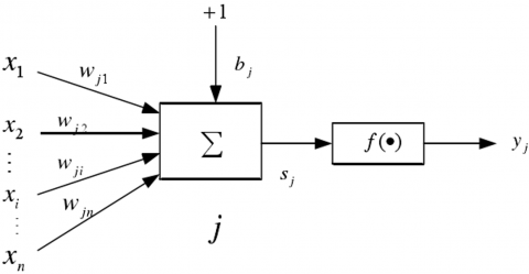
The BPNN algorithm consists of the forward propagation of data (the forward calculating of data) and the reverse propagation of error signal (the reverse calculation of error). The typical structure of the BPNN has three layers: an input layer, a hidden layer, and an output layer. The information is imported to the input layer, transmitted to the hidden layer, and eventually to the output layer. Each layer has one or multiple nodes. The training results are saved by connecting the stored weights and thresholds between nodes. Figure 1 is the sketch map of node j in the BPNN.
Figure 1. The sketch map of a node in the BPNN
Note: $x_{i}$ is the input of node $i ; w_{i j}$ is connection weight between nodes $i$ and $j ; b_{i}$ is the threshold of node $j ; f(\cdot)$ is the transfer function; $y_{j}$ is the output of node $j ; S_{j}$ is the input of node $j$
The input of node j Sj can be defined as:
$S_{j}=\sum_{i=1}^{n} w_{i j} * x_{i}+b_{j}=W_{j} X+b_{j}$ (15)
where, $X=\left[x_{1}, x_{2}, \ldots, x_{i}, \ldots, x_{n}\right]^{T}$;
$w_{j}=\left[w_{j 1}, w_{j 2}, \ldots w_{j i}, \ldots, w_{j n}\right]$.
2.2 Preprocessing of customer complaint data
This paper takes the total number of work orders in response to future customer complaints in a power enterprise as the prediction target. According to business regulations of the power enterprise, 25 secondary work orders, denoted as x1,x2,…,x25 , were adopted as the initial independent variables of the prediction model, and combined into the experimental data (real number of customer complaints) (as shown in Table 1).
Table 1. The experimental data
|
Data |
x1 |
x2 |
… |
x25 |
|
2019/7/17 |
6 |
7 |
… |
11 |
Considering the different types of customer complaints and the features of ARIMA time series algorithm, the sample period was set as October 28, 2016 - September 30, 2019. For MLP and BPNN algorithms, the total number of complaints in a week was taken as the dependent variable, and the sample period was set s July 2018 – September 2019.
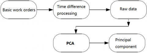
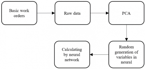
Before modeling, the independent variables of 25 dimensions were preprocessed through principal component analysis (PCA) [14] (Figure 2) to reduce the dimensionality of the experimental data (independent variables). The preprocessing was designed to overcome the following defects of the BPNN and MLP algorithms.
For the BPNN algorithm, the network training will be disrupted by the strong correlations between the multiple dimensions of independent variables, because the NN boasts strong non-mapping ability. For the MLR algorithm, it is too complex and unstable to select independent variables for the prediction model, if the 25 dimensions are directly analyzed through the MLR. Besides, the algorithm will face a high error due to the multicollinearity among variables.
Figure 2. The workflow of data preprocessing
To determine the data preprocessing rules, the time difference index of the secondary work orders was calculated by:
$\left|\hat{y}_{c}(l)-y_{c}\right|=\min \left\{\left|f_{1}\left(x_{c}\right)-y_{c}\right|, \mid f_{2}\left(x_{c}\right)\right.$$\left.-y_{c} \mid, \ldots,\right\}, l \in[L, c-L]$ (16)
where, $t$ is the current time; $n$ is the time difference between the dependent variable and independent variables; $\hat{y}_{c}(n)$ is the predicted value of the dependent variable with time difference of $n ; f_{n}\left(x_{c}\right)$ is the prediction function with time difference $n$ $L$ is the best time difference between the dependent variable and independent variables.
The PCA function [15] was adopted to quantify the amount of information contained in the experimental data, and derive the proportion of retained features. Through the PCA, the original 25 dimensions of experimental data were reduced, producing 25 principal components zi. The contribution rate of each principal component is given in Table 2.
As shown in Table 2, the cumulative contribution rate of the top 10 principal components was greater than the standard of 95%. Therefore, the top 10 principal components were selected for modeling. The 10 independent variables composed of the original variables are denoted as $z_{1}, z_{2}, z_{3}, \ldots, z_{10}$. The post-PCA data are real numbers (Table 3).
Table 2. The contribution rate of each principal component
|
Principal component |
Contribution rate |
Principal component |
Contribution rate |
|
z1 |
5.2327316e-01 |
z14 |
1.7367937e-33 |
|
z2 |
2.4017867e-01 |
z15 |
1.1953031e-33 |
|
z3 |
1.2418776e-01 |
z16 |
4.2185412e-34 |
|
z4 |
3.0221702e-02 |
z17 |
1.4989573e-34 |
|
z5 |
2.2126571e-02 |
z18 |
1.2835612e-34 |
|
z6 |
5.3771892e-03 |
z19 |
9.2564128e-35 |
|
z7 |
3.8396812e-03 |
z20 |
7.3239296e-35 |
|
z8 |
2.8772871e-03 |
z21 |
5.8510517e-35 |
|
z9 |
2.4376591e-03 |
z22 |
1.9598416e-35 |
|
z10 |
1.1693662e-03 |
z23 |
1.0441226e-35 |
|
z11 |
3.9589887e-04 |
z24 |
4.6101328e-36 |
|
z12 |
2.5808767e-04 |
z25 |
3.5857562e-36 |
|
z13 |
1.5285181e-32 |
|
|
Table 3. The post-PCA data
|
Data |
z1 |
z2 |
… |
z10 |
|
2019/7/17 |
6 |
7 |
… |
3 |
2.3 Three prediction models
The ARIMA time series prediction model was constructed by the steps in Figure 3.
Figure 3. The construction steps of ARIMA time series prediction model
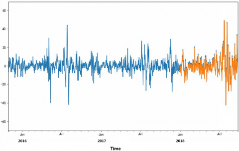
Figure 4. The comparison between the predicted results and the actual data of ARIMA time series prediction model
The time series of each Monday was chosen as experimental data to verify the accuracy of the ARIMA (p, d, q) customer complaint prediction model in predicting the number of complaints in the coming week. The parameters of the model were configured as p=2, d=1, and q=2. Figure 4 compares the predicted results with the actual data.
As shown in Figure 4, the time series fluctuated through the sample period, and the curve of predicted value agreed well with the curve of the real value. The two curves exhibited very similar volatility. Although the prediction results are reasonable, the ARIMA time series prediction model only applies to short-term prediction, failing to achieve a good fitting effect in the long run.
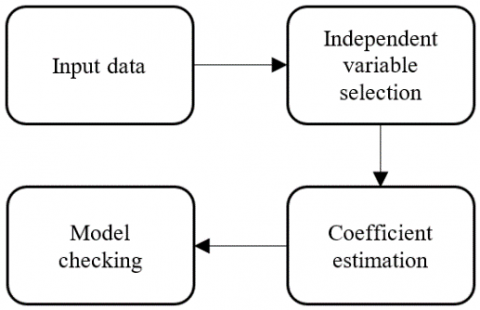
The MLR aims to solve the MLR equation based on the relationship between a dependent variable and multiple independent variables. The ARIMA time series prediction model was constructed by the steps in Figure 5.
Figure 5. The construction steps of MLR prediction model
The establishment of the MLR equation is essentially to estimate the coefficient of the MLR model and look for a suitable expression. In the MLR prediction model, the parameter vectors were estimated by the least squares (LS) method. The basic idea of solving the MLR equation is to calculate the partial regression coefficient in the MLR model by the LS principle, so as to minimize the sum of squares of the residual errors between the observed values and the regression values. After the MLR model was established, the MLR fitting equation was obtained as:
$y=0.133 x_{1}+0.72 x_{2}+0.201 x_{3}-1.652 x_{4}$$\quad+0.602 x_{5}-3.468 x_{6}-0.93 x_{7}$$-13.419 x_{8}-1.17 x_{9}+0.94 x_{10}$-2.31 (17)
Figure 6 compares the predicted results with the actual data.
Figure 6. The comparison between the predicted results and the actual data of MLR prediction model
As shown in Figure 6, the actual value and predicted value had basically the same trend, but with a large error between them. Thus, the MLR prediction model has a poor predictive effect: the model cannot effectively regress and summarize the complex relationship between independent variables and the dependent variable.
The BPNN prediction model was constructed by the steps in Figure 7.
Figure 7. The construction steps of BPNN prediction model
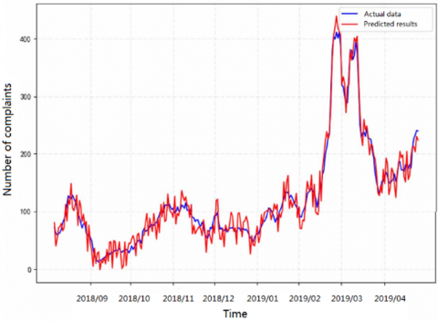
Figure 8. The comparison between the predicted results and the actual data of BPNN prediction model
In this experiment, the principal components of the original data after dimensionality reduction were taken as the independent variables (inputs) of the prediction, and the total number of customer complaints in the coming week was taken as the dependent variable (output). Since 10 principal components were selected through the PCA, the BPNN has a total of 10 input layer nodes.
Even if the parameters remain constant, the BPNN algorithm might output different weights to the model, and make different predictions in each run. To solve the problem, the BPNN algorithm was ran 200 times. The ten minimum and ten maximum results were removed. Then, the remaining 180 results were averaged as the final prediction. Figure 8 compares the predicted results with the actual data.
As shown in Figure 8, the predicted value was almost identical with the actual value, an evidence of the ultrahigh accuracy of the BPNN algorithm.
Table 4 compares the relative errors of the three prediction models.
Table 4. The relative errors of the three prediction models
|
Model |
Relative error<10% |
Relative error<30% |
|
ARIMA |
34.36% |
86.02% |
|
MLR |
25.87% |
68.76% |
|
BPNN |
75.31% |
89.82% |
It can be seen from Table 4 that the BPNN prediction model achieved much higher accuracy than the other two models. Judging by prediction accuracy and fitness between dependent and independent variables, the BPNN algorithm is clearly the best algorithm to build the customer complaint prediction model.
One of the most prominent defects of the BPNN is the random selection of weights and thresholds. This problem could be effectively overcome by the GA [16, 17]. The principle of GA-optimization of BPNN is as follows: First, the GA selects an encoding method for the weights and thresholds of BPNN, and generates an initial population with a certain number of individuals [18]. Then, a fitness function is defined as per the optimization objective to calculate the fitness of each individual. Based on the fitness, the next generation population is established through genetic operations. Through iterative evolution, the individuals with the best fitness are selected.
Here, a GA is designed in four steps: determining the encoding method; selecting the fitness function; performing genetic operations (selection, crossover, and mutation); identifying the important parameters. Let N be the initial population. Then, the design of the GA can be explained as follows:
(1) Determining the encoding method
The real number method was selected as the encoding method, because it can contain all the weights and thresholds of the BPNN. Specifically, each individual was regarded as a real string, which consists of four parts: the connection weight between hidden and output layers, the connection weight between input and hidden layers, the threshold of the hidden layer, and the threshold of the output layer.
To illustrate the encoding of weights and thresholds, a simple BPNN of 2 input layer nodes, 2 hidden layer nodes, and 1 output layer node was established as an example. Firstly, the BPNN generates a sequence with a length of 9 and a numerical range of (- 1,1). Then, the individuals are encoded as [0.1, 0.2, 0.3, 0.4, 0.5, 0.6, 0.7, 0.8, 0.9]. The weights and thresholds of the BPNN are given in Figure 9.
Figure 9. The encoding of the BPNN
(2) Determining the fitness function
In this research, the individuals refer to the initial weights and thresholds of the BPNN. Therefore, the individuals were brought into the BPNN as the initial values of weights and thresholds. After the network is trained, the samples were tested in the trained network. If the error of the test sample is small, the individual was considered superior. Therefore, the fitness function was defined as the sum of the absolute errors between the predicted output and the expected output:
$F=\sum_{i=1}^{n} a b s\left(y_{i}-o_{i}\right)$ (18)
where, n is the number of output layer nodes; yi is the expected output of the i-th node; oi is the predicted output of the i-th hidden layer node.
(3) Performing genetic operations
Step 1. Selection
The selection aims to select individuals with relatively high fitness. Here, the roulette selection [19] is performed to select individuals. Let N be the population size, fi be the fitness of individual xi , and F be the total fitness. Then, the selection probability can be calculated by:
$p_{i}=f_{i} / \sum_{i=1}^{N} f_{i}$ (19)
The fitness of individual xi can be calculated by:
$f_{i}=k / F$ (20)
Step 2. Crossover
First, two individuals were selected by roulette method. Then, the genes in the chromosomes of the two individuals were swapped at a certain probability for cross validation. The real number crossover was selected, because our research chooses real number encoding.
Step 3. Mutation
The mutation alters the value of a gene or multiple genes at a small probability, such that the population is diverse enough and the individuals are of high quality.
Step 4. Identifying important parameters
The important parameters include the initial population size, crossover probability, mutation probability, maximum number of iterations, to name but a few. These parameters have a great impact on the prediction results. At present, there is not yet a way to accurately determine the optimal value of each parameter. The parameter values need to be adjusted through repeated experiments [20]. In this paper, the initial population size is set to 100, the maximum number of iterations to 200, the crossover probability to 0.75, and the mutation probability to 0.2.
Under the above settings, the GA-BPNN customer complaint prediction model was adopted to predict the number of customer complaints from July 2018 to September 2019. Through 200 iterations, the optimal fitness of individuals was obtained at 0.0637. The corresponding individuals were selected as the initial weights and thresholds of the BPNN.
Figure 10 compares the actual value with the value predicted by BPNN and that predicted by GA-BPNN. As shown in Figure 10, the GA-BPNN prediction model achieved the better prediction effect. Table 5 compares the relative errors between the GA-BPNN and BPNN models.
As shown in Table 5, the GA-BPNN model was more accurate than the BPNN model, indicating that the GA can optimize the performance of the BPNN to a certain extent.
Figure 10. The comparison between the predicted results of two models and the actual data
Table 5. The relative errors between the GA-BPNN and BPNN models
|
Model |
Relative error<10% |
Relative error<30% |
|
BPNN |
75.31% |
89.82% |
|
GA-BPNN |
76.27% |
95.32% |
This paper analyzes and implements three common customer complaint prediction models. Through comparison, the BPNN model was found to be the most accurate. However, the BPNN algorithm is easy to fall into the local minimum, which lowers the prediction accuracy. To solve the problem, the BPNN customer complaint prediction model was optimized by the GA. Specifically, the original population was encoded and initialized, and subject to selection, crossover, and mutation. In this way, the initial weights, and thresholds of the BPNN were optimized. Then, the optimized BPNN was trained and then applied to predict the customer complaints in the near future. The GA-BPNN model provides an effective tool to rationalize the staffing of customer service department and prevent potential customer complaints in the power industry.
[1] Montoya, F.G., Baños, R., Gil, C., Espín, A., Alcayde, A., Gómez, J. (2010). Minimization of voltage deviation and power losses in power networks using Pareto optimization methods. Engineering Applications of Artificial Intelligence, 23(5): 695-703. https://doi.org/10.1016/j.engappai.2010.01.011
[2] Dragičević, T., Wheeler, P., Blaabjerg, F. (2018). Artificial intelligence aided automated design for reliability of power electronic systems. IEEE Transactions on Power Electronics, 34(8): 7161-7171. https://doi.org/10.13140/RG.2.2.34206.18246
[3] Wang, H.F., Zhang, C.Y., Lin, D.Y., He, B.T. (2019). An artificial intelligence based method for evaluating power grid node importance using network embedding and support vector regression. Frontiers of Information Technology & Electronic Engineering, 20(6): 816-828. https://doi.org/10.1631/FITEE.1800146
[4] Yu, S., Zhu, K., Diao, F. (2008). A dynamic all parameters adaptive BP neural networks model and its application on oil reservoir prediction. Applied Mathematics and Computation, 195(1): 66-75. https://doi.org/10.1016/j.amc.2007.04.088
[5] Ling, M.H., Tsui, K.L., Balakrishnan, N. (2014). Accelerated degradation analysis for the quality of a system based on the gamma process. IEEE Transactions on Reliability, 64(1): 463-472. https://doi.org/10.1109/TR.2014.2337071
[6] Miao, X., Hao, Y., Zhang, F., Zou, S., Ye, S., Xie, Z. (2020). Spatial distribution of heavy metals and their potential sources in the soil of Yellow River Delta: a traditional oil field in China. Environmental Geochemistry and Health, 42(1): 7-26. https://doi.org/10.1007/s10653-018-0234-5
[7] Wang, Y., Wang, C., Shi, C., Xiao, B. (2018). Short-term cloud coverage prediction using the ARIMA time series model. Remote Sensing Letters, 9(3): 274-283. https://doi.org/10.1080/2150704X.2017.1418992
[8] Chen, C.K., Shie, A.J., Yu, C.H. (2012). A customer-oriented organisational diagnostic model based on data mining of customer-complaint databases. Expert Systems with Applications, 39(1): 786-792. https://doi.org/10.1016/j.eswa.2011.07.074
[9] Grégoire, Y., Laufer, D., Tripp, T.M. (2010). A comprehensive model of customer direct and indirect revenge: Understanding the effects of perceived greed and customer power. Journal of the Academy of Marketing Science, 38(6): 738-758. https://doi.org/10.1007/s11747-009-0186-5
[10] Sun, G., Bin, S., Jiang, M., Cao, N., Zheng, Z., Zhao, H., Xu, L. (2019). Research on Public Opinion Propagation Model in Social Network Based on Blockchain. CMC-Computers Materials & Continua, 60(3): 1015-1027. https://doi.org/10.32604/cmc.2019.05644
[11] Mistry, P., Neagu, D., Trundle, P.R., Vessey, J.D. (2016). Using random forest and decision tree models for a new vehicle prediction approach in computational toxicology. Soft Computing, 20(8): 2967-2979. https://doi.org/10.1007/s00500-015-1925-9
[12] Lyu, M.N., Yang, Q.S., Yang, N., Law, S.S. (2016). Tourist number prediction of historic buildings by singular spectrum analysis. Journal of Applied Statistics, 43(5): 827-846. https://doi.org/10.1080/02664763.2015.1078302
[13] Yadav, A.K., Chandel, S.S. (2014). Solar radiation prediction using Artificial Neural Network techniques: A review. Renewable and Sustainable Energy Reviews, 33: 772-781. https://doi.org/10.1016/j.rser.2013.08.055
[14] Sun, G., Bin, S. (2018). A new opinion leaders detecting algorithm in multi-relationship online social networks. Multimedia Tools and Applications, 77(4): 4295-4307. https://doi.org/10.1007/s11042-017-4766-y
[15] Peng, Z., Jiang, Y., Yang, X., Zhao, Z., Zhang, L., Wang, Y. (2018). Bus arrival time prediction based on PCA-GA-SVM. Neural Network World, 28(1): 87-104. https://doi.org/10.14311/NNW.2018.28.005
[16] Gong, D., Sun, J., Miao, Z. (2016). A set-based genetic algorithm for interval many-objective optimization problems. IEEE Transactions on Evolutionary Computation, 22(1): 47-60. https://doi.org/10.1109/TEVC.2016.2634625
[17] Aziza, H., Krichen, S. (2018). Bi-objective decision support system for task-scheduling based on genetic algorithm in cloud computing. Computing, 100(2): 65-91. https://doi.org/10.1007/s00607-017-0566-5
[18] Bin, S., Sun, G., Cao, N., Qiu, J., Zheng, Z., Yang, G., Xu, L. (2019). Collaborative Filtering Recommendation Algorithm Based on Multi-Relationship Social Network. CMC-Computers Materials & Continua, 60(2): 659-674. https://doi.org/10.32604/cmc.2019.05858
[19] Qin, Q., Cheng, S., Zhang, Q., Li, L., Shi, Y. (2015). Particle swarm optimization with interswarm interactive learning strategy. IEEE Transactions on Cybernetics, 46(10): 2238-2251. https://doi.org/10.1109/TCYB.2015.2474153
[20] Sun, G., Bin, S. (2018). Construction of learning behavioral engagement model for MOOCs platform based on data analysis. Educational Sciences: Theory & Practice, 18(5): 2206-2216. https://doi.org/10.12738/estp.2018.5.120