Akram Esvand Rahmani* | Moosa Katouli
© 2020 IIETA. This article is published by IIETA and is licensed under the CC BY 4.0 license (http://creativecommons.org/licenses/by/4.0/).
OPEN ACCESS
Given that breast cancer is one of the most difficult and dangerous cancers, the use of diagnostic methods in the early stages of its development can be very effective and important in the process of treating patients. This early diagnosis can help doctors treat patients, thus greatly reducing mortality. Many different features have been collected to diagnose and predict breast cancer, and it is very difficult for specialists to use all of these features for a large number of cancers. The aim of this study is to provide a new method for minimizing the process of breast cancer diagnosis through the Grasshopper optimization algorithm. The steps of the proposed method consist of three main parts: The first step after receiving the data is to normalize the pre-processed data. The second step is to reduce the features using the GOA. The final step is to select the optimal features and improve the parameters using the SVM Classifier. The experiments in this study were performed on three datasets, namely WBC (Wisconsin Breast Cancer), WDBC (Wisconsin Diagnosis Breast Cancer) and WPBC (Wisconsin Prognosis Breast Cancer). The results show that the accuracy of the proposed method is 99.51, 98.83 and 91.38 for the WBC, WDBC and WPBC datasets, respectively. In comparison with other methods, the results show that the proposed method has better performance.
breast cancer, classification SVM, diseases, grasshopper optimization algorithm
Breast cancer is one of the most common diseases in women, the timely diagnosis of which plays an important role in the continuation of life and treatment. Therefore, knowing the basic information in this area is necessary for every woman, even if she does not have the disease.
Breast cancer is a tumor, in which the cells of the breast tissue begin to divide and develop due to genetic disorders such as mutation, chromosomal aberration, deletion, reorganization, chromosomal translocation and replication [1]. In fact, not all tumors are cancerous and they may be benign or malignant. Benign tumors grow abnormally, but are rarely fatal [2]. However, a number of benign breast masses can also increase the risk of breast cancer. Moreover, some women with a history of benign breast biopsy have a higher risk of breast cancer. On the other hand, malignant tumors are more serious and may be cancerous, but early detection of these cancers has increased the chance of successful treatment. one of the methods early detection and disease classification is data mining [3].
Data mining in health care is a very important branch in diagnosis and in deeper understanding of medical data. Medical health data mining is about solving real-world problems in diagnosis and treatment of diseases [4].
Understanding preventive and therapeutic approaches to diseases such as breast cancer is possible through data mining. This method has a prominent role in the patterns identification of tools and many other methods for data mining and analysis which have implemented similar algorithms. Researchers use different methods and algorithms with different perception and accuracy to diagnose breast cancer that being not very accurate, as well as working with large datasets cause major problems which result in a very long processing time. Therefore, eliminating unnecessary features while retaining important ones can help to increase the accuracy of the proposed method.
Due to the fact that the reduction methods of the features that have been utilized in other studies are not highly recognizable and suffer from local optimality from local optimization in methods such as PSO and genetics, a method of reducing the new feature has been used in this study.
The proposed method uses Grasshopper Optimization Algorithm (GOA) to select the optimal features. the purpose of this study, in addition to improve the accuracy of classification, is prevention and early detection of breast cancer using the new and hybrid method of GOA and Support Vector Machine (SVM) classification which is going to be discussed in the following sections.
The structure of the present manuscript is as follows: the second section presents a review of known methods of breast cancer diagnosis. The third section presents the methodology and method of dimensionality diagnosis in breast cancer. The fourth section evaluates the methods examined along with the results and their comparison and analysis, and the conclusions are presented in the fifth section.
Since breast cancer is one of the most difficult and dangerous cancers, applying diagnostic methods in the early stages of its development can be very effective in the patient’s treatment. So far, many algorithms have been developed for the diagnosis of breast cancer and different challenges are addressed. These methods are reviewed in this section.
In 2016, Asri et al. [5], used machine learning algorithms to predict and classify the WBC (original) dataset. In this experiment, different clusters such as SVM, decision tree C4.5, Naive Bayes and KNN nearest neighbor were evaluated. The accuracy of SVM in this experiment with Weka tool was 97.13. The purpose of evaluating these methods is to compare the accuracy and efficiency of the employed algorithms.
Chowdhary et al. [6], have used mammography images to diagnose breast cancer. In the used method, the intuitive fuzzy histogram magnification method was used to process the data which improves the images. In the next step, the probabilistic Fuzzy Clustering method was used to segment and separate the cancerous tissues. Therefore, this method allows processing in large cancerous issue datasets, as well as the main purpose which is providing better accuracy in the separation of breast cancer tissues. In the following step, the matrix methods of gray area coefficient and linear binary pattern were used to extract the textural properties. The accuracy of this method was 94%. This method is not only highly selective, but also hard to handle with large datasets, which in addition to extending the processing time, sometimes even makes it possible to model datasets for them.
Another method which was used by Aalaei et al. [7] for classification of breast cancer metastases was the use of genetic meta-specificity reduction method. The experiment was performed on three different datasets of WBC, WDBC and WPBC using Artificial Neural Network (ANN) cluster. The accuracy of the proposed method was estimated for WBC, WDBC and WPBC to be 96, 96.1 and 76.3, respectively. In this method, although the feature is reduced, the accuracy of the method can be improved to a relatively small extent.
In 2017, Nilashi et al. [8] presented a knowledge-based system using fuzzy logic method. This method consists of three steps: the first step is the processing of Wisconsin Breast Cancer (original) data. Data clustering is then performed in similar groups using the Expectation Maximization (EM) clustering method in the second step. After the feature reduction by PCA, the fuzzy rule set is finally classified into data using a regression tree in the last step. The accuracy of this method was obtained using WBCD dataset to be 93.2. Adopting learning rules for datasets can sometimes complicate the classification task.
In another method [9], the Bat algorithm was used to select the optimal features of breast cancer for diagnosis. In this method, 286 samples from the WDBC dataset were selected using simple random sampling to choose the features. After the feature selection, the overall ranking was performed based on the similarity for classification by Random Forest (RF). The accuracy of this method was considered to be 96.85. Selecting samples at random can sometimes make the process of selecting features difficult.
In a study by Doreswamy et al. [10], an improved method based on the Bat algorithm was presented for classification of breast cancer. In this study, binary Bat algorithm was used. The accuracy of the proposed method for the training set and test set was 92.61 and 89.95 respectively. UCI data on 569 samples was used in the experiment.
In 2018, a study by Muslim [11] presented a method using PSO to reduce the specificity to diagnose breast cancer. The purpose of this method is to determine the level of breast cancer. Diagnosis is performed on 699 samples of the UCI dataset after pre-processing and reducing the specificity using the PSO algorithm by categorizing the decision tree C4.5 into two categories. The category deals with malignant and benign. The accuracy of the proposed method was 95.61%.
Recently, a combination approach by Sahu et al. [12] has classified and diagnosed breast cancer. Using the PCA feature reduction method, this method has used different clusters, as well as ANN classification with 97% best performance among other clusters. The experiments were performed on 699 samples containing 9 features with two benign and malignant labels.
Although the results of previous studies are an important step in diagnosis of breast cancer, each of methods has some weaknesses, such as elimination of unreported data in data analysis.
The method of diagnosis and classification of breast cancer by the GOA has not been tested and evaluated in three different breast cancer datasets. The strengths of the present study include reducing detection costs, utilizing better performance classification without the adverse effects of aggressive methods, high detection accuracy compared to the cited papers, selection of titles commensurate with available data and complete comparison with the previous researches. In the proposed method, after optimization of data, pre-processing and data normalization, the optimized and desirable features are selected by the GOA. Then, the SVM classification with the optimal parameters is discussed.
The steps of the proposed method consist of three main parts: the first step, after receiving the data, is to normalize the pre-processed data. The second step is to reduce the features using the GOA. The final step is to select the optimal features and improve the parameters using the SVM cluster, which ultimately results in classification of the data into two benign and malignant categories.
3.1 Grasshopper Optimization Algorithm (GOA)
Optimization methods suffer from falling into local optimal locations because the algorithm considers a local optimal solution instead of the global optimal solution so it would not be able to find the global optimal features [13].
Therefore, the locust algorithm or the GOA is a new meta-algorithm that attempts to find optimal answers to complex mathematical and even real-world problems by mimicking the locusts' behavior in nature to find food [13].
${{\text{X}}_{\text{i}}}\text{=}{{\text{S}}_{\text{i}}}\text{+}{{\text{G}}_{\text{i}}}\text{+}{{\text{A}}_{\text{i}}}$ (1)
This algorithm is inspired by the flight path of locust in nature: the $\mathrm{X}_{\mathrm{i}}$ denotes the position of the ith grasshopper, Si is the social interaction, $G_{i}$ is the gravitational force on the ith grasshopper, $A_{i}$ is the horizontal force on the direction of the ith grasshopper’s movement. Since social interaction is the main search mechanism in the GOA which is computed as follows:
$S_{i}=\sum_{j=1, j \neq i}^{N} s\left(d_{i j}\right) \hat{d}_{i j}$ (2)
In relation to (1), $\mathrm{d}_{\mathrm{ij}}$ is the distance between ith and jth grasshopper which is calculated as $d_{\mathrm{ij}}=\left|x_{j}-\mathrm{x}_{i}\right|$. In addition, $\hat{d}_{\mathrm{ij}}$ is a singular vector from the ith grasshopper to the jth grasshopper which is calculated as $\hat{d}_{\mathrm{ij}}=\frac{x_{j}-{\mathrm{x}_{i}}}{d_{\mathrm{ij}}}$ [13].
Given the visibility of the principal component S in Eq. (1), the direction of the locust in the congestion is defined as the follows:
$s(r)=f e^{\frac{-r}{l}}-e^{-r}$ (3)
where, f is the gravity intensity and l represents the scale of gravity length of the social interaction. Hence, the amplitude occurs in [0.2, 079] [14], which is the situation when the locust is at a distance of 2,079 units from the adjacent locust; no attractions or repulsions exists. This area is referred to as the comfort zone (Figure 1).
Figure 1. The behavior pattern among the Grasshoppers [14]
The components G and A represent the gravitational force of the locust and the horizontal force of the wind, respectively, which are obtained by Eqns. (4) and (5):
$G_{i}=-g \widehat{e_{g}}$ (4)
In Eq. (4), g is the gravitational constant and $\widehat{\mathrm{e}_{\mathrm{g}}}$ is a singular vector towards the center of the Earth.
$A_{i}=u \widehat{e_{w}}$ (5)
where, u is the constant of drift and $\widehat{e_{w}}$ is a singular vector in the wind direction.
The locust optimization algorithm was mathematically corrected by Saremi et al. [13] as the follows:
$X_{i}^{d}=c\left(\sum_{j=1, j \neq i}^{N} c \frac{u b_{d}-l b_{d}}{s} s\left(\left|x_{j}^{d}-x_{i}^{d}\right|\right) \frac{x_{j}-x_{i}}{d_{i j}}+{\widehat{T}}_{d}\right.$ (6)
where, $u b_{d}$ and $l b_{d}$ are the upper and lower limit in d respectively, ${\widehat{T}}_{d}$ is the best solution and c is the subtraction coefficient to reduce the comfort, repulsion and gravity areas.
In Eq. (6), $\frac{u b_{d}-l b_{d}}{s}$ is a term that linearly reduces the space which grasshoppers need for exploration and exploitation, and $s\left(\left|x_{j}^{d}-x_{i}^{d}\right|\right)$ indicates whether a grasshopper should be repelled from the target or absorbed into it. Parameter c is the controller of the GOA which is computed as follows:
$c=\operatorname{cmax}-l \frac{\operatorname{cmax}-\operatorname{cmin}}{L}$ (7)
In Eq. (7), cmax and cmin represent the maximum and minimum values of c, respectively.
3.2 Support Vector Machine (SVM)
The kernel methods, one of which is a support vector machine, are essentially divided into two parts: (a) the part that maps the input data into the vector space, which is called the feature space; and (b) the learning algorithm which detects the linear patterns in the desired attribute. The input data are being written using the kernel functions in a feature space on a larger scale, so that the similarity criteria can be determined based on the internal parameters. The linear categorization is described only based on the internal parameters of the data. The support vector categorization is expressed as follows:
$f(x)=\beta_{0}+\sum_{i=1}^{n} \alpha_{i}\left\langle x, x_{i}\right\rangle, i=1, \ldots, n$ (8)
In this function, a parameter, $\alpha_{i}$, is defined for each object. The internal result between each of the xi training objects and the new object x must be computed. If the training object is not a support vector, $\alpha_{i}$ will be zero. If S is the desired support vector, the solution function will be as the follows:
$f(x)=\beta_{0}+\sum_{i \in S} \alpha_{i}\left\langle x, x_{i}\right\rangle$ (9)
Therefore, only domestic products are needed to draw the linear classifier f(x) and calculate its coefficients. K is the kernel function for determination of their similarities. The linear kernel is similar to support vector clustering and applies where $\left(\mathrm{x}_{\mathrm{i}}, \mathrm{x}_{\mathrm{i}^{*}}\right)=\sum_{\mathrm{j}}^{\mathrm{p}} \mathrm{x}_{\mathrm{ij}} \mathrm{x}_{\mathrm{i}^{*} \mathrm{j}}$. The linear kernel determines the similarity between the two results by Pearson's correlation method. Polynomial cores and radial cores are two examples of the most commonly used cores. The radial nucleus is also commonly referred to as the Radial Basis Function (RBF) nucleus or the Gaussian radial base nucleus. From now on, for the purpose of this study, only the term “radial core” is used. The polynomial of degree, d, is presented in the following section. In this equation, d is the kernel parameter (positive integer). If d equals 1, then the kernel is linear:
$\mathrm{K}\left(\mathrm{x}_{\mathrm{i}}, \mathrm{x}_{\mathrm{j}}\right)=\left(1+\sum_{\mathrm{j}=1}^{\mathrm{p}} \mathrm{x}_{\mathrm{ij}} \mathrm{x}_{\mathrm{i}, \mathrm{j}}\right)^{\mathrm{d}}$ (10)
The radial core is expressed as follows:
$\mathrm{K}\left(\mathrm{x}_{\mathrm{i}}, \mathrm{x}_{\mathrm{j}}\right)=\left\{-\gamma \sum_{\mathrm{j}=1}^{\mathrm{p}}\left(\mathrm{x}_{\mathrm{ij}} \mathrm{x}_{\mathrm{i}, \mathrm{j}}\right)^{2}\right\}$ (11)
In this equation, γ is the kernel parameter and a positive constant.
3.3 Feature reduction by GOV-SVM
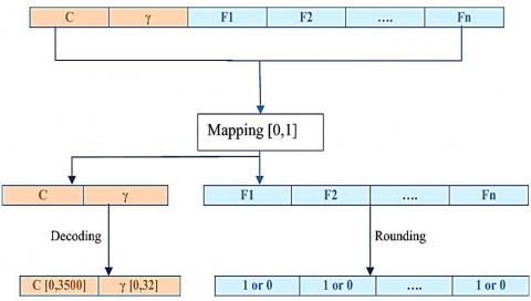
In the proposed method, the proposed feature selection method by Ibrahim et al. [15] is used for feature reduction. Accordingly, the samples are encrypted using a vector of real numbers. This vector consists of two parts: the first part contains the cost part, C, and the gamma parameter, "γ", and the second part contains the selected features. Therefore, C and "γ" are being normalized in the intervals of [0, 3500] and [0, 32]. Eq. (12) shows such a normalization:
$Y=\frac{X-m i n_{X}}{\operatorname{man}_{X}-\min _{X}}\left(\operatorname{man}_{Y}-\min _{Y}\right)+\min _{Y}$ (12)
The second part is used for those features which are in the interval of [0, 1]. As shown in the upper part of Figure 2, if the component value is greater than or equal to 0.5, it is replaced by 1, which indicates a feature is selected; otherwise, the approximate value is 0 and that means this feature is not selected.
Figure 2. Data mapping and decoding [15]
Therefore, the proposed SVM + GOA system for reducing the feature can be stated as follows:
$\mathrm{FB}=\frac{\mathrm{FA}-\mathrm{min}_{\mathrm{FA}}}{\max _{\mathrm{FA}}-\min _{\mathrm{FA}}}$ (13)
$\mathrm{ACC}=\frac{\mathrm{T}_{\mathrm{P}}+\mathrm{T}_{\mathrm{N}}}{\mathrm{T}_{\mathrm{P}}+\mathrm{F}_{\mathrm{N}}+\mathrm{F}_{\mathrm{p}}+\mathrm{T}_{\mathrm{N}}}$ (14)
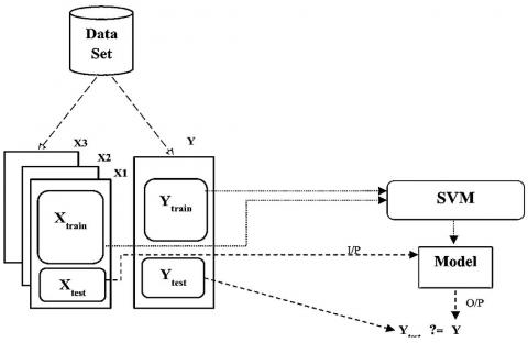
The proposed SVM + GOA flowchart [15] of feature selection is shown in Figure 3, which depicts the relationship among the main sections.
Figure 3. Defining training and test sets [15]
This section presents the results of implementation and trials of the proposed method for diagnosis of breast cancer. Experiments have been carried out on the methods by MATLAB 2019ra software and Windows 10 as the operating system with Corei5 processor and 4 GB main memory.
4.1 Dataset
The proposed method uses three different datasets. The first dataset contains the data from the UCI dataset, comprising 699 samples that fall into eight groups [16]. The first, second, third, fourth, fifth, sixth, seventh and eighth group includes 367, 71, 31, 17, 48, 49, 31 and 86 samples, respectively [17]. These data now include 10 Codi bacterial attributes: cell thickness, cell shape uniformity, cell size uniformity, marginal adhesion, single epithelial cell size, nude nucleus, chromatin, normal nucleus and mitosis, which are divided into benign and malignant.
The second set of data includes 569 samples which are obtained from the Wisconsin Hospital. This dataset consists of 569 samples including 367 benign patients and 212 malignant patients. This dataset from the UCI website is categorized into benign and malignant. These attributes include:
The third dataset contains 198 samples including 34 attributes that are classified into two categories of recur and non-recur which is provided from the UCI website. These attributes include:
In Table 1, it shows summary details of the used dataset in the proposed method.
Table 1. Summary details of the used dataset in the proposed method [7]
|
Dataset |
Number of Attributes |
Number of Instances |
Number of class |
|
Wisconsin breast cancer (WBC) |
11 |
699 |
2 |
|
Wisconsin diagnosis breast cancer (WDBC) |
32 |
569 |
2 |
|
Wisconsin prognosis breast cancer (WPBC) |
34 |
198 |
2 |
4.2 Evaluation criteria
The Breast dataset is divided into training and test dataset. The training dataset for the SVM classifier consists of 70% of the total dataset, and the test dataset consists of 30% of the total data. The proposed method is effectively compared to PSO [11], GA [7], Bat [9] and PCA [12] in terms of performance metrics which are obtained by the following Equations [18]:
$\mathrm{Accuracy}=\frac{\mathrm{T}_{\mathrm{p}}+\mathrm{T}_{\mathrm{N}}}{\mathrm{N}}$ (15)
Specificity $=\frac{\mathrm{T}_{P}}{\mathrm{T}_{\mathrm{p}}+F_{\mathrm{N}}}$ (16)
sensitivity $=\frac{\mathrm{T}_{P}}{\mathrm{T}_{P}+F_{\mathrm{N}}}$ (17)
where, TN is the number of True Negatives, TP is the number of True Positives, FN is the number of False Negatives and FP is the number of False Positives [19].
4.3 Goa parameters selection
In the experiments, the number of iterations for the grasshopper optimization algorithm is set to be 200. In addition, parameter values cMAX = 2.079 and cMIN = 0.00004 are considered.
4.4 Investigation of the proposed method
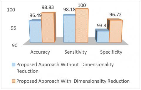
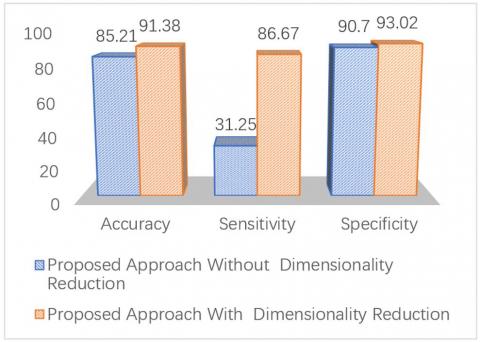
In this subsection, the results of the experiments are reported. The results of the experiments on various datasets, including WBC, WDBC and WPBC, with and without of feature reduction are shown in Figures 4, 5 and 6.
Figure 4. The proposed method on the WBC dataset
Figure 5. The proposed method on the WDBC dataset
Figure 6. The proposed method on the WPBC dataset
As shown in Figures 4, 5, and 6, the criteria of accuracy, sensitivity, and specificity show better performance in all three datasets when the dimensions are reduced. The features selected in all three sets using the GOA method are listed in Table 2. Considering the selected features in Table 2, the following features are used to compare the proposed method to PSO, GA, Bat and PCA methods.
Table 2. The selected features after applying feature selection method
|
Dataset |
Number features |
Selected features |
|
WBC |
3 |
3,5,10 |
|
WDBC |
8 |
5,6,7,20,22,24,25,28 |
|
WPBC |
15 |
5,9,10,11,12,18,19,20,24,25,26,27,31,33,34 |
4.5 Comparison of the proposed method with other methods
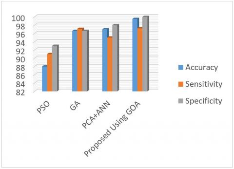
In this subsection, the proposed method is first compared to the other meta-heuristic methods, such as PSO, GA and Bat, and then the PCA feature reduction method is used to detect WBC datasets (Figure 7 and Table 3).
As shown in Table 3 and Figure 7, the proposed method performs better than the other methods. In the methods such as GA and PSO which suffer from local optimization problem, the accuracy is lower. In PCA feature selection method, despite the good training by neural network hidden layers, the performance is still weaker than the proposed method. It should be noted that the test is performed after removing incomplete records, namely 683 records.
The flowing, is Compared the proposed method with other methods using WDBC and WPBC datasets. Tables 4, 5 and Figure 8 and 9.
As shown in Table 4 and Figure 8, the proposed method performs better than the GA and BBA methods while being very close to the PSO method. The GA method is in the third place despite the improvement of the parameters. The BBA method, which is an improved binary form of Bat method, is the weakest method compared to the others.
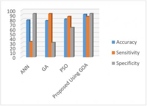
According to Table 5 and Figure 9, the performance of the proposed method is better than the other methods and is significantly less sensitive than the PSO method. The GA method is better than the proposed method using the WPBC dataset in terms of sensitivity. However, in other datasets the WBC and WDBC perform more strongly. The ANN method also performs poorly compared to the other methods
Table 3. Comparison of the proposed method with other methods using WBC dataset
|
Method |
Accuracy |
Sensitivity |
Specificity |
|
PSO [11] |
88.00 |
91.00 |
93.00 |
|
GA [7] |
96.6 |
97.1 |
96.6 |
|
PCA+ANN [12] |
97.00 |
95.00 |
98.00 |
|
Proposed Using GOA |
99.51 |
97.23 |
100 |
Table 4. Comparison of the proposed method with other methods using WDBC dataset
|
Method |
Accuracy |
Sensitivity |
Specificity |
|
BBA [20] |
92.61 |
91.98 |
88.80 |
|
GA [7] |
96.6 |
97.5 |
93.7 |
|
PSO [7] |
97.2 |
98 |
95.6 |
|
Proposed Using GOA |
98.83 |
100 |
96.72 |
Table 5. Comparison of the proposed method with other methods using WPBC dataset
|
Method |
Accuracy |
Sensitivity |
Specificity |
|
ANN [7] |
79.2 |
33 |
92.9 |
|
GA [7] |
78.1 |
92.8 |
31.0 |
|
PSO [21] |
81.3 |
86.9 |
63.2 |
|
Proposed Using GOA |
91.38 |
86.67 |
93.02 |
Figure 7. Comparison of the proposed method with other methods using WBC dataset
Figure 8. The proposed method on the WDBC dataset
Figure 9. The proposed method on the WPBC dataset
In this study, a breast cancer detection method based on Grasshopper optimization is presented on three WBC, WDBC and WPBC datasets. The proposed Grasshopper-based approach is mathematically modeled and mimics the Grasshopper group behavior in nature to solve the optimization problems. The proposed grasshopper-based method selects a subset of optimized features that are classified by SVM into two categories. Then, the proposed method is compared to the other methods based on GA, PSO, ANN and PCA algorithms. The results show that the proposed method is able to predict and diagnose breast cancer on three datasets and its quantitative performance results are superior to the other methods. Since the method of detecting breast cancer with the GOA has not been investigated so far, it can be further investigated with other feature selection methods and other classifications, such as SVM, C4.5 and naïve Bayes.
[1] Ashkhaneh, Y., Mollazadeh, J., Aflakseir, A., Goudarzi, M., Homaei Shandiz, F. (2015). Study of difficulty in emotion regulation as a predictor of incidence and severity of nausea and vomiting in breast cancer patients. Fundamentals of Mental Health, 3: 125-131. https://pdfs.semanticscholar.org/35d3/b6c9302ee1e3ef72a02ec192372a25d1e023.pdf.
[2] Sharifian, A., Pourhoseingholi, M.A., Emadedin, M., Rostami Nejad, M., Ashtari, S., Hajizadeh, N., Firouzei, S.A., Hosseini, S.J. (2015). Burden of breast cancer in Iranian women is increasing. Asian Pacific Journal of Cancer Prevention, 16(12): 5049-52. https://doi.org/10.7314/apjcp.2015.16.12.5049
[3] Matsumoto, A., Jinno, H., Ando, T., Fujii, T., Nakamura, T., Saito, J., Takahashi, M., Hayashida, T., Kitagawa, Y. (2016). Biological markers of invasive breast cancer. Japanese Journal of Clinical Oncology, 46(2): 99-105. https://doi.org/10.1093/jjco/hyv153
[4] Williams, K., Adebayo Idowu, P., Ademola Balogun, J., Oluwaranti, A. (2015). Breast cancer risk prediction using data mining classification techniques. Transactions on Networks and Communications, 3(2): 1-11. https://doi.org/10.14738/tnc.32.662
[5] Asri, H., Mousannif, H., AlMoatassime, H., Nodel, H. (2016). Using machine learning algorithms for breast cancer risk prediction and diagnosis. Procedia Computer Science, 83: 1064-1069. https://doi.org/10.1016/j.procs.2016.04.224
[6] Chowdhary, C.L., Acharjya, D.P. (2016). Breast cancer detection using intuitionistic fuzzy histogram hyperbolization and possibilitic fuzzy c-mean clustering algorithms with texture feature based classification on mammography images. AICTC '16: Proceedings of the International Conference on Advances in Information Communication Technology & Computing, pp. 1-6. https://doi.org/10.1145/2979779.2979800
[7] Aalaei, S., Shahraki, H., Rowhanimanesh, A., Eslami, S. (2016). Feature selection using genetic algorithm for breast cancer diagnosis: Experiment on three different datasets. Iran J Basic Med Sci., 19(5): 476-482.
[8] Nilashia, M., Ibrahima, O., Ahmadic, H., Shahmoradi, L. (2017). A knowledge-based system for breast cancer classification using fuzzy logic method. Telematics and Informatics, 34(4): 133-144. https://doi.org/10.1016/j.tele.2017.01.007
[9] Jeyasingh, S., Veluchamy, M. (2017). Modified bat algorithm for feature selection with the wisconsin diagnosis breast cancer (WDBC) dataset. Asian Pacific Journal of Cancer Prevention, 18(5): 1257-1264. https://doi.org/10.22034/APJCP.2017.18.5.1257
[10] Doreswamy, H., Salma M.U. (2016). A binary bat inspired algorithm for the classification of breast cancer data. International Journal on Soft Computing, Artificial Intelligence and Applications (IJSCAI), 5(2/3): 1-21. https://doi.org/10.5121/ijscai.2016.5301
[11] Muslim, M., Hardiyanti, S., Sugiharti, E., Prasetiyo, B., Alimah, S. (2018). Optimization of C4.5 algorithm-based particle swarm optimization for breast cancer diagnosis. International Conference on Mathematics, Science and Education 2017 (ICMSE2017), Semarang, Indonesia, pp. 1-7. https://doi.org/10.1088/1742-6596/983/1/012063
[12] Sahu, B., Nandan, S., Mohanty, Kumar Rout S. (2019). A hybrid approach for breast cancer classification and diagnosis. EAI Endorsed Transactions on Scalable Information Systems, 6: 1-8. https://doi.org/10.4108/eai.19-12-2018.156086
[13] Saremi, S., Mirjalili, S., Lewis, A. (2017). Grasshopper Optimisation Algorithm: Theory and application. Advances in Engineering Software, 105: 30-47. https://doi.org/10.1016/j.advengsoft.2017.01.004
[14] Aljarah, I., Al-Zoubi, A.M., Faris, H., Hassonah, A.M., Mirjalili, S., Saadeh, H. (2018). Simultaneous feature selection and support vector machine optimization using the grasshopper optimization algorithm. Cognitive Computation, 10: 478-495. https://doi.org/10.1007/s12559-017-9542-9
[15] Ibrahim, T.H., Mazher, W.J., Ucan, O.N., Bayat, O. (2018). A grasshopper optimizer approach for feature selection and optimizing SVM parameters utilizing real biomedical data sets. Neural Computing and Applications, 31: 5965-5974. https://doi.org/10.1007/s00521-018-3414-4
[16] Zeeshan, M., Salam, B., Khalid, Q.S.B., Alam, S., Sayani, R. (2018). Diagnostic accuracy of digital mammography in the detection of breast cancer. Cureus, 10(4): e2448. https://doi.org/10.7759/cureus.2448
[17] UCI Machine Learning Repository: Breast Cancer Wisconsin (Diagnostic) Data Set [Internet]. Archive.ics.uci.edu. 2016 [cited 12 May 2016]. Available from: http://archive.ics.uci.edu/ml/datasets/Breast+Cancer+Wisconsin+%28Diagnostic%29, accessed on 16 December, 2019.
[18] Breast Cancer Wisconsin (Original) Data Set Available from:https://archive.ics.uci.edu/ml/datasets/breast+cancer+wisconsin+%28original%29, accessed on 16 December, 2019.
[19] Tahmooresi, M., Afshar, A., Bashari Rad, B., Nowshath, K. (2018). Early detection of breast cancer using machine learning techniques. Journal of Telecommunication, Electronic and Computer Engineering, 10: 21-27.
[20] Mafarja, M.M., Mirjalili, S. (2017). Whale Optimization Algorithm with simulated annealing for feature selection. Neurocomputing, 260: 302-312. https://doi.org/10.1016/j.neucom.2017.04.053
[21] Sakri, S.B., Abdul Rashid, B.N., Muhammad Zain, Z. (2018). Particle swarm optimization feature selection for breast cancer recurrence prediction. IEEE Access, 6: 29637-29647. https://doi.org/10.1109/ACCESS.2018.2843443