Saravana Moorthy Anusha![]() | Singaram Athithan*
| Singaram Athithan*![]()
© 2024 The authors. This article is published by IIETA and is licensed under the CC BY 4.0 license (http://creativecommons.org/licenses/by/4.0/).
OPEN ACCESS
Over the past three decades, there has been a notable increase in the occurrence of diabetes. The International Diabetes Federation (IDF) states that in 2021, over 537 million individuals worldwide have been diagnosed with diabetes. Here, we derive a stochastic model with white noise (incidence rate fluctuation, treatment efficacy variability, behavioral factors, and environmental influence) to study the dynamics of type 2 diabetes. Since the dynamics of stochastically perturbed models are substantially different from those of deterministic models, stochastic models provide an additional degree of realism to real-world problems for epidemic diseasesFurthermore, we broadened our deterministic model by transforming it into an optimal control model and subjected it to analysis using Pontryagin's Maximum Principle. In addition, we have performed a numerical simulation, which may serve as a verification of our theoretical research findings. Consequently, we conclude that an elevation in the transition rate from susceptible to imbalanced glucose levels results in an increase in the treatment and restrain population of the stochastic model.
type 2 diabetes, stochastic mathematical model, optimal control analysis, white noise
As per the World Health Organization (WHO), diabetes is a chronic medical condition marked by hyperglycemia. This occurs either due to insufficient insulin secretion from the pancreas or resistance to insulin within the body [1]. The prominent signs and indicators of diabetes are frequent urination, blurred vision, thirst, dry mouth, weight loss, tiredness, and slow-healing wounds. Also, diabetes is associated with several risk factors, including heart attack, high blood pressure, blindness, and poor sleep quality.
The International Diabetes Federation (IDF) reports that there are over 1.2 million individuals globally diagnosed with type 1 diabetes; one-sixth (21 million) of live births are affected by diabetes during pregnancy; nearly 966 billion dollars were spent on healthcare; about 6.7 million deaths were caused by diabetes: over 240 million individuals were living with diabetes are undiagnosed, more than 537 million individuals with diabetes in 2021, This number is projected to rise to 643 million by 2030 and is anticipated to further escalate to 783 million by 2045 [2].
In recent years, several mathematical models have been developed to investigate the characteristics of diabetes [3-7]. Some of them are, a model structured by age for complications associated with diabetes [8], an optimal control model for managing the diabetes population [9], obesity increases the susceptibility of individuals to develop type 2 diabetes. [10] and effect of physical exercise [11].
Conversely, Pinto and Carvalho [12] formulated a mathematical model to assess the clinical consequences of the concurrent presence of diabetes and tuberculosis. Moreover, Nath et al. [13] have discussed the importance of control-oriented meal models and insulin dynamics. And reviewed briefly about the progress in the creating of knowledge-driven blood glucose dynamic models. Moreover, Kouidere et al. [14] presented a deterministic model examining the coexistence of COVID-19 and diabetes. They utilized an optimal control model to identify the adverse impact of quarantine on individuals with diabetes amid the COVID-19 pandemic.
Specifically, Anusha and Athithan [15]’s work indicates that the model is taken into account in the space $\mathbb{R}_4^{+}$, which divided the model into diabetes susceptible class S(t), Imbalance Glucose Level(IGL) class I(t), treatment class T(t) and restrain class R(t). At the time t, the total population sizes is given by N(t)=S(t)+I(t)+T(t)+R(t). The differential equations are as follows:
$\begin{aligned} & \frac{d S}{d t}=\Lambda-\alpha S-\mu S+\ell R \\ & \frac{d I}{d t}=\alpha S-\beta I-\rho I T-\mu I \\ & \frac{d T}{d t}=\beta I+\rho I T-\gamma T-\mu T \\ & \frac{d R}{d t}=\gamma T-\mu R-\ell R\end{aligned}$ (1)
where, Λ represents the recruitment rate of S, α is the rate of progression of individuals from S to I, β represents the progression rate from I to T, ρ denotes the interaction rate between IGL and treatment population, $\ell$ is the rate at which individuals who have recovered lose their immunity, γ represents the recovered rate, and μ indicates the natural demise rate. It is presumed that all parameter values are positive constants. For model (1), there exist two non-negative equilibria namely:
• Diseases Free Equilibrium (DFE) $E^{(0)}=\left(S^0, I^0, T^0, R^0\right)=\left(\frac{\Lambda}{\alpha+\mu}, 0,0,0\right)$.
• Endemic Equilibrium (EE) E1=(S*, I*, T*, R*) where,
$\begin{gathered}S^*=\frac{I^* \beta \ell \gamma+\Lambda k_3 k_4-I^* \Lambda k_4 \rho}{k_1 k_4\left(k_3-I^* \rho\right)}, \\ T^*=\frac{I^* \beta}{\left(k_3-I^* \rho\right)^{\prime}} \\ R^*=\frac{I^* \beta \gamma}{k_4\left(k_3-I^* \rho\right)}, \\ I_1^*=\frac{-G_2+\sqrt{G_2^2-4 G_1 G_3}}{2 G_1} .\end{gathered}$
where, $\quad k_1=\alpha+\mu, k_2=\beta+\mu, k_3=\gamma+\mu, k_4=\mu \ell, G_1=$ $\mu \rho k_1 k_4, G_2=-\left(\alpha \Lambda k_4 \rho+k_5\right), G_3=\Lambda \alpha k_3 k_4$. Further, by employing the "next-generation matrix method" the treatment reproduction number $R_T$ for our deterministic model (1) is calculated as:
$R_T=\frac{\rho}{\gamma+\mu} I^*$,
which denotes the potential treatment level after the IGL population enters the treatment compartment. And the positive invariant set for our deterministic model (1) is as follows:
$\Omega=\left\{(S, I, T, R) \in \mathbb{R}_{+}^4: S>0, I>0, T>0, R>0,0<S+I+T+R \leq \frac{\Lambda}{\mu}.\right\}$
Further, it is important to note that all the mathematical models for diabetes mentioned above are deterministic in nature. The random movements of population fluctuation, individual death rate, immigration rate, and other complications are ignored. Since the deterministic model has few restrictions in biological systems, we cannot predict the dynamics of diabetes more accurately. Therefore, the implement of randomness in the model (1) changes it to the stochastic differential equations which offer a more realistic approach to studying epidemic diseases [16-21].
For example, Rajalakshmi and Ghosh [22] suggest that the virotherapy success rate is relatively higher in the stochastic diffenrential model than in the deterministic model. In particular, Yuan and Allen [23] used stochastic model to investigate the dynamics of viruses and immune systems. Furthermore, Srivastav et al. [24] showed that, in a stochastic simulation, the criminal population level is notably less than the estimated value generated by the corresponding deterministic model.
Motivated by the aforementioned works, we are extending the deterministic model proposed by Anusha and Athithan [15] to a stochastic model, since stochastic models have a greater capacity to capture the random variations present in the diabetes under consideration. Furthermore, a model for optimal control is created, leading to the derivation of mathematical results from it [25-27].
The remaining of this article is organized as: In Section 2, we extend model (1) by considering the effects of stochasticity; In Section 3, performing optimal control to identify key parameters for managing diabetes; In Section 4, we performed some numerical experiments to validate the analytical results; Section 5 provides a summary of our results.
We will extend the model (1) to a stochastic one, recognizing that stochastic models are better suited for capturing the inherent random fluctuations in the biological dynamics of the diabetes.
The development of a stochastic model follows the methodology introduced by Yuan and Allen [23]. Let the random variable Z(t)=(Z1(t), Z2(t), Z3(t), Z4(t))H be continuous for (S(t), I(t), T(t), R(t))H where the transpose of matrix is denoted by H.
The random vector represents the change in random variables during the time interval $\Delta t$ is represented by ΔZ=Z(t+Δt)-Z(t)=(ΔZ1, ΔZ2, ΔZ3, ΔZ4)H. We will now delineate the transition maps that articulate all conceivable state changes within the stochastic model. Derived from our deterministic model (1), it becomes evident that there are 11 potential state changes within a small time interval Δt. Table 1 presents a discussion on state changes and their corresponding probabilities.
Consider a scenario where a susceptible human transitions to an infected state due toIGL. In this instance, the state change ΔZ is represented as ΔZ=(-1, 1, 0, 0) its probability of the occurrence is expressed as:
$\begin{gathered}\operatorname{Prob}\left\{\left(\Delta Z_1, \Delta Z_2, \Delta Z_3, \Delta Z_4\right)=(-1,1,0,0) \mid\left(Z_1, Z_2, Z_3, Z_4\right)\right\} \\ =P_2=\alpha Z_1 \Delta t+o(\Delta t) .\end{gathered}$
The determination of the change in expectation E(ΔZ) and its covariance matrix V(ΔZ) related with ΔZ by disregarding terms bigger than o(Δt). The expectation of ΔZ is expressed as follows:
$E(\Delta Z)=\sum_{i=1}^{11} P_i(\Delta Z)_i \Delta t=\left(\begin{array}{l}\Lambda-\alpha S-\mu S+\ell R \\ \alpha S-\beta I-\rho I T-\mu I \\ \beta I+\rho I T-\gamma T-\mu T \\ \gamma T-\mu R-\ell R\end{array}\right) \Delta t=f\left(Z_1, Z_2, Z_3, Z_4\right) \Delta t$.
It should be noted that in this context, both the function f and the expectation vector maintain the similar structure as those observed in the model (1).
Further the covariance matrix V(ΔZ)=E((ΔZ)(ΔZ)H)-E(ΔZ)(E(ΔZ)H) and E((ΔZ)(ΔZ)H)=f(Z)(f(Z)H)Δt, it can be approximated with diffusion matrix ɸ times Δt byslighting the term of (Δt)2 such that V(ΔZ)≈E((ΔZ)(ΔZ)H).
Hence
$\begin{gathered}E\left((\Delta Z)(\Delta Z)^H\right)=\sum_{i=1}^{11} P_i\left((\Delta Z)_i(\Delta Z)_i^H\right) \Delta t= \\ \left(\begin{array}{llll}V_{11} & V_{12} & 0 & V_{14} \\ V_{21} & V_{22} & V_{23} & 0 \\ 0 & V_{32} & V_{33} & V_{34} \\ V_{41} & 0 & V_{43} & V_{44}\end{array}\right) \cdot \Delta t=\phi \cdot \Delta t,\end{gathered}$
In this context, the aforementioned diffusion matrix is positive-definite and symmetric. The derivation of each element of this 4×4 diffusion matrix is given:
$\begin{gathered}V_{11}=P_1+P_2+P_3+P_4=\Lambda+\alpha Z_1+\mu Z_1+\ell Z_4, \\ V_{12}=V_{21}=-P_2=-\alpha Z_1, V_{14}=V_{41}=-P_4=-\ell Z_4, \\ V_{22}=P_2+P_5+P_6+P_7=\alpha Z_1+\beta Z_2+\rho Z_2 Z_3+\mu Z_2, \\ V_{23}=V_{32}=-P_5-P_6=-\beta Z_2-\rho Z_2 Z_3, \\ V_{33}=P_5+P_6+P_8+P_9=\beta Z_2+\rho Z_2 Z_3+\gamma Z_3+\mu Z_3, \\ V_{34}=V_{43}=-P_8=-\gamma \\ V_{44}=P_4+P_8+P_{10}=\ell Z_4+\gamma Z_3+\mu Z_4,\end{gathered}$
Table 1. Potential state transitions and their related probabilities
|
Possible Stage Change |
|
Probability of State Changes |
|
$(\Delta Z)_1=(1,0,0,0)^H$ |
Change when the recruitment increases. |
$P_1=\Lambda \Delta t+o(\Delta t)$ |
|
$(\Delta Z)_2=(-1,1,0,0)^H$ |
Change when some individuals moves from susceptible compartment to IGL compartment. |
$P_2=\alpha Z_1 \Delta t+o(\Delta t)$ |
|
$(\Delta Z)_3=(-1,0,0,0)^H$ |
Mortality rate of susceptible class. |
$P_3=\mu Z_1 \Delta t+o(\Delta t)$ |
|
$(\Delta Z)_4=(1,0,0,-1)^H$ |
Change when some recovered individual moves to susceptible class. |
$P_4=\ell Z_4 \Delta t+o(\Delta t)$ |
|
$(\Delta Z)_5=(0,-1,1,0)^H$ |
Change when some individuals moves from IGL class to treatment class. |
$P_5=\beta Z_2 \Delta t+o(\Delta t)$ |
|
$(\Delta Z)_6=(0,-1,1,0)^H$ |
Change when there is an interaction between IGL class and treatment class. |
$P_6=\rho Z_2 Z_3 \Delta t+o(\Delta t)$ |
|
$(\Delta Z)_7=(0,-1,0,0)^H$ |
Mortality rate of IGL class. |
$P_7=\mu Z_2 \Delta t+o(\Delta t)$ |
|
$(\Delta Z)_8=(0,0,-1,1)^H$ |
Change when some individuals Moves from treatment compartment to restrain compartment. |
$P_8=\gamma Z_3 \Delta t+o(\Delta t)$ |
|
$(\Delta Z)_9=(0,0,-1,0)^H$ |
Mortality rate of treatment class. |
$P_9=\mu Z_3 \Delta t+o(\Delta t)$ |
|
$(\Delta Z)_{10}=(0,0,0,-1)^H$ |
Mortality rate of restrain class. |
$P_{10}=\mu Z_4 \Delta t+o(\Delta t)$ |
|
$(\Delta Z)_{11}=(0,0,0,0)^H$ |
No change. |
$P_{11}=\left(1-\sum_{i=1}^{10} P_i\right)+o(\Delta t)$ |
We adhere to the approach outlined by Yuan and Allen [23] and generate a matrix Q in such a way that ɸ=QQH, where Q is a 4×9 matrix.
$K=\left(\begin{array}{lllllllll}\sqrt{P_1+P_3} & \sqrt{P_2} & \sqrt{P_4} & 0 & 0 & 0 & 0 & 0 & 0 \\ 0 & -\sqrt{P_2} & 0 & \sqrt{P_5} & \sqrt{P_6} & \sqrt{P_7} & 0 & 0 & 0 \\ 0 & 0 & 0 & -\sqrt{P_5} & -\sqrt{P_6} & 0 & \sqrt{P_8} & \sqrt{P_9} & 0 \\ 0 & 0 & -\sqrt{P_4} & 0 & 0 & 0 & -\sqrt{P_8} & 0 & \sqrt{P_{10}}\end{array}\right)$
Therefore, Ito stochastic differential model holds the subsequent form:
$d(Z(t))=f\left(Z_1, Z_2, Z_3, Z_4\right) d t+Q . d W(t)$
with initial condition Z(0)=(Z1(0), Z2(0), Z3(0), Z4(0))H and W(t)=((W1(t), W2(t), W3(t), W4(t), W5(t), W6(t), W7(t), W8(t), W9(t))H is a Wiener process,.
Taking into account the aforementioned information, we form the stochastic model in the following manner:
$\begin{aligned} d S & =[\Lambda-\alpha S-\mu S+\ell R] d t+\sqrt{\Lambda+\mu S} d W_1+\sqrt{\alpha S} d W_2+\sqrt{\ell R} d W_3 \\ d I & =[\alpha S-\beta I-\rho I T-\mu I] d t-\sqrt{\alpha S} d W_2+\sqrt{\beta I} d W_4+\sqrt{\rho I T} d W_5+\sqrt{\mu I} d W_6, \\ d T & =[\beta I+\rho I T-\gamma T-\mu T] d t-\sqrt{\beta I} d W_4-\sqrt{\rho I T} d W_5+\sqrt{\gamma T} d W_7+\sqrt{\mu T} d W_8, \\ d R & =[\gamma T-\mu R-\ell R] d t-\sqrt{\ell R} d W_3-\sqrt{\gamma T} d W_7+\sqrt{\mu R} d W_9 .\end{aligned}$ (2)
Here, we extend our deterministic model to an optimal control model since optimal control theory has emerged as a promising tool for minimizing the overall number of infectives within a finite time span while minimizing the effort cost. In examining this model, we will apply Pontryagin’s Maximum Principle [28-31]. The ensuing expression represents the formulated optimal control system along with the objective functional:
$\begin{aligned} \frac{d S}{d t} & =\Lambda-\alpha S-\mu S+\ell R, \\ \frac{d I}{d t} & =\alpha S-\beta I-\rho(t) I T-\mu I, \\ \frac{d T}{d t} & =\beta I+\rho(t) I T-\gamma(t) T-\mu T, \\ \frac{d R}{d t} & =\gamma(t) T-\mu R-\ell R.\end{aligned}$ (3)
3.1 The optimal control problem
We employ optimal control theory to analyze the dynamics of the provided model. The objective functional, for a fixed time tf, is expressed as follows:
$J=\int_0^{t_f}\left(C_1 I+\frac{1}{2} C_2 \rho^2+\frac{1}{2} C_3 \gamma^2\right) d t$ (4)
in compliance with the state system provided by (3). Here, the parameter C1≥0, C2≥0, C3≥0 and they symbolize the weight constants.
Our aim is to ascertain the control parameters ρ* & γ*, such that:
$J\left(\rho^*, \gamma^*\right)=\min _{\rho, \gamma \in \Gamma} J(\rho, \gamma)$,
where, Γ represents the control set and is defined as Γ={ρ, γ: measurable and 0≤ρ(t), γ(t)≤1} and $t \epsilon\left[0, t_f\right]$.
The Lagrangian problem is termed as $L(I, \rho, \gamma)=C_1 I+\frac{1}{2} C_2 \rho^2+\frac{1}{2} C_3 \gamma^2$.
In addressing our problem, we formulate the Hamiltonian $\mathcal{H}$ in the following manner:
$\mathcal{H}(I, \rho, \gamma)=L(I, \rho, \gamma)+\lambda_1 \frac{d S}{d t}+\lambda_2 \frac{d I}{d t}+\lambda_3 \frac{d T}{d t}+\lambda_4 \frac{d R}{d t}$,
where, λi, i=1, 2, 3, 4 are the co-state\adjoint variables and can be found by solving the model (5):
$\begin{aligned} & \frac{d \lambda_1}{d t}=-\frac{\partial \mathcal{H}}{\partial S}=\alpha\left(\lambda_1-\lambda_2\right)+\mu \lambda_1, \\ & \frac{d \lambda_2}{d t}=-\frac{\partial \mathcal{H}}{\partial I}=-C_1+(\beta+\rho T)\left(\lambda_2-\lambda_3\right)+\mu \lambda_2, \\ & \frac{d \lambda_3}{d t}=-\frac{\partial \mathcal{H}}{\partial T}=\left(\lambda_2-\lambda_3\right) \rho I+\gamma\left(\lambda_3-\lambda_4\right)+\mu \lambda_3, \\ & \frac{d \lambda_4}{d t}=-\frac{\partial \mathcal{H}}{\partial R}=\ell\left(\lambda_4-\lambda_1\right)+\mu \lambda_4,\end{aligned}$ (5)
Let $\tilde{S}, \tilde{I}, \tilde{T}$ and $\tilde{R}$ be the optimal value of S, I, T and R. Additionally, let {λ1, λ2, λ3, λ4} be the solutions of the model (5).
3.2 Optimal control theorems
In modelling, optimal control strategies are applied to model and manage the spread of diseases. By optimizing intervention measures such as vaccination campaigns or quarantine protocols [31], public health officials can better control and alleviate the repercussions of infectious diseases [32].
Theorem 3.1 There exist optimal controls $\rho^*, \gamma^* \in \Gamma$ in such a way that $J\left(\rho^*, \gamma^*\right)=\min _{\rho, \gamma \rightarrow \Gamma} J(\rho, \gamma)$ subject to system (3).
Proof. Lenhart and Workman's model (2007), outlined in "Optimal control applied to biological models," applies optimal control theory to optimize biological systems, offering insights for effective decision-making in areas such as disease management and resource allocation [32]. It is easy to see that all the the state variables and the control are non-negative. For this minimization problem, the requisite convexity of our objective function in ρ and γ is also verified. The control variable set $\rho, \gamma \epsilon \Gamma$ is also closed and convex by definition. Furthermore, the integrand in the functional (4), $C_1 I+\frac{1}{2} C_2 \rho^2+\frac{1}{2} C_3 \gamma^2$ is bounded and convex on the control set Γ, as well as for the state variables. Atlast, the theorem is proved.
Given the presence of an optimal control to reduce the function under the constraints of Eqs. (3) and (5), the optimal solution can be acquired through the use of Pontryagin's Maximum Principle. The sufficeint conditions can be derived in the following manner:
Let (x, u) be an optimal solution to an optimal control problem. Then, there exists a non trivial vector function λ=(λ1, λ2, ..., λn) that satisfies the following equalities.
$\begin{aligned} \frac{d x}{d t} & =\frac{\partial H(t, x, u, \lambda)}{\partial \lambda}, \\ 0 & =\frac{\partial H(t, x, u, \lambda)}{\partial u}, \\ \frac{d \lambda}{d t} & =-\frac{\partial H(t, x, u, \lambda) .}{\partial x}\end{aligned}$ (6)
Utilizing Theorem 3.1 alongside the Pontryagin’s Maximum Principle [33], our aim is to introduce and clarify the following theorem.
Theorem 3.2 The optimal controls $\rho^*, \gamma^*$ minimizes $\mathbf{J}$ over the region $\Gamma$ defined by $\rho^*=\max \{0, \min (\tilde{\rho}, 1)\}$ and $\gamma^*=$ $\max \{0, \min (\tilde{\gamma}, 1)\}$, where, $\rho=\frac{\tilde{I} \tilde{T}\left(\widetilde{\lambda_2}-\widetilde{\lambda_3}\right)}{c_2}, \gamma=\frac{\tilde{T}\left(\widetilde{\lambda_3}-\widetilde{\lambda_4}\right)}{c_3}$.
Proof. By applying the optimality conditions $\frac{\partial H}{\partial \rho}=0$ and $\frac{\partial H}{\partial \gamma}=0$, we get $\frac{\tilde{I} \tilde{T}\left(\widetilde{\lambda_2}-\widetilde{\lambda_3}\right)}{C_2}, \gamma=\frac{\tilde{T}\left(\widetilde{\lambda_3}-\widetilde{\lambda_4}\right)}{C_3}$.
These controls have upper and lower boundaries of $0 \& 1$ respectively. That is $\rho=0$ if $\tilde{\rho}<0 \& \rho=1$ if $\tilde{\rho}>1 \& \gamma=0$ if $\tilde{\gamma}<$ $0 \& \gamma=1$ if $\tilde{\gamma}>1$, apart from that $\rho=\tilde{\rho} \& \gamma=\tilde{\gamma}$. Therefore for this controls $\left(\rho^*\right) \&\left(\gamma^*\right)$ the optimal value of the functional $\mathbf{J}$, as defined in Eq. (4), is determined, hence proved.
We carried out numerical experiments for the model (2) by applying the Euler-Maruyama method. We assumed that all the parameters are in years. Now, choosing the parameter values of the system as:
$\begin{gathered}Y_1=(\Lambda, \alpha, \rho, \beta, \gamma, \mu, \ell)= (100,0.0099,0.000009,0.0199,0.0170,0.0167,0.0009) .\end{gathered}$
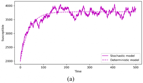
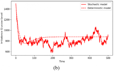
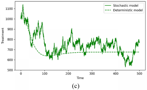
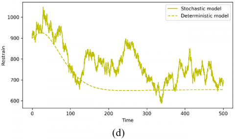
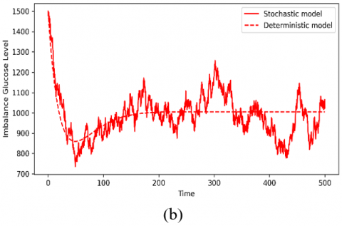
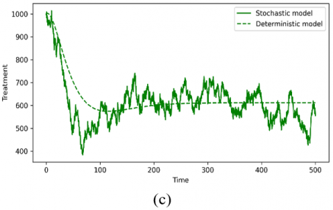
For this parameter set, model (1) and (2) has the EE point which is stable. Further, Figure 1 depicts the comparison outcomes of the model (1) and model (2) for the parameter set, and the mean of the 500 runs is plotted. It is observed that the dynamics of the susceptible population are similar for both models. However, the stochastic simulation of IGL, treatment and restrain population are little deviate from the corresponding deterministic simulation.
Subsequently, we choose the following set of parameters:
$\begin{gathered}Y_2=(\Lambda, \alpha, \rho, \beta, \gamma, \mu, \ell)= (100,0.0099,0.000009,0.0150,0.0170,0.0167,0.0009) .\end{gathered}$
For this set of numerical values, we obtain the unique EE point for the model (1) and (2) which is shown in Figure 2. From the Figure, it is noticed that the simulation of the stochastic model (2) is quite close to the model (1).
Figure 1. Time evolutions of (a) susceptible population, (b) IGL population, (c) treatment population, and (d) restrain population for model (1) and model (2) using the parameter set Y1
Figure 2. Time evolutions of (a) susceptible population, (b) IGL population, (c) treatment population, and (d) restrain population for model (1) and model (2) using the parameter set Y2
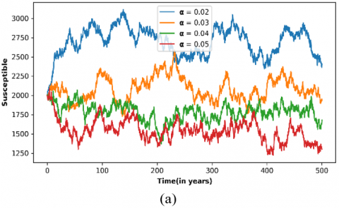
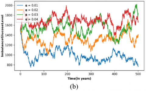
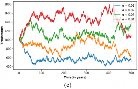
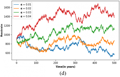
Figure 3. Variation of (a) susceptible population, (b) IGL population, (c) treatment population, and (d) restrain population for stochastic model (2) with respect to time for various values of α and other parameters as in Y2
The causes of diabetes are still an unpredictable phenomenon in most people, and therefore it is essential to include environmental effects like the behavior of individuals, and genetic and lifestyle factors as white noise in the deterministic model to study stochasticity. This motivates us to study stochastic perturbation in the physical world problem. Here, a deterministic model is improved by introducing environmental noise effects into the stochastic model to make the system can handle more practical circumstances.
We studied the simulation results of both models after transitioning the model (1) to a stochastic model (2). For the parameter set Y1, the results obtained from the stochastic model suggest a less number of IGL population in comparison to the outcomes of the corresponding deterministic model. However, for parameter Y2, the simulation results of the stochastic model closely resembles those of the deterministic model.
Here we had considered the white noise terms which represents the physical and mental dilemma of every human being due to the environmental/situation changes that occur in society. Based on this fact only the evolution of stochasticity has been started and it goes beyond our level of thinking nowadays. The rise and fall of the population in each of our compartments are not only based on the individual’s dilemma alone. It is the effect created by decision-makers in any group or society. It’s harder to specify any reason for that.
Even small suggestions in the advertisements about the reduction of diabetes may develop a concern about that in any individual/group of people’s mindset. In that sense, we may say that there may be many reasons for such kinds of fluctuations here and there for producing the effect among each compartment. These fluctuations were effectively depicted in Figures 1-2. These visuals were exhibiting a particular effect on the population.
Finally, we conclude that there are many fluctuations among the population of diabetes based on the white noise level arrangement or natural arousement of situations. Also, we would like to comment on the fact that if the progression rate from susceptible to IGL is high then the probability of the IGL population will become higher as shown in Figure 3. Our findings illustrate that the stochastic model gives an additional dimension to the diabetes epidemic model. In our forthcoming research, we intend to incorporate Levy noise and telegraph noise into the deterministic model.
Blood glucose levels can exhibit random fluctuations influenced by factors such as physical activity, diet, stress, and other environmental variables. Including Lévy noise in mathematical models helps researchers capture and understand the stochastic nature of these fluctuations.
[1] Roglic, G. (2016). WHO global report on diabetes: A summary. International Journal of Noncommunicable Diseases, 1(1): 3. https://www.who.int/publications/i/item/9789241565257
[2] International Diabetes Federation. (2021). IDF Diabetes Atlas, 10th Ed. Brussels, Belgium. https://www.diabetesatlas.org.
[3] Mollah, S., Biswas, S. (2021). Effect of awareness program on diabetes mellitus: deterministic and stochastic approach. Journal of Applied Mathematics and Computing, 66: 61-86. https://doi.org/10.1007/s12190-020-01424-6
[4] Agarwal, M., Pathak, R. (2014). The impact of awareness programs by media on the spreading and control of non-communicable diseases. International Journal of Engineering, Science and Technology, 6(5): 78-87. https://doi.org/10.4314/ijest.v6i5.7
[5] Mwita, P.S., Shaban, N., Mbalawata, I.S., Mayige, M. (2021). Mathematical modelling of root causes of hyperglycemia and hypoglycemia in a diabetes mellitus patient. Scientific African, 14: e01042. DOI:https://doi.org/10.1016/j.sciaf.2021.e01042
[6] Ma, H., Xiao, J., Chen, Z., Tang, D., Gao, Y., Zhan, S., Keir, M.Y.A. (2021). Relationship between helicobacter pylori infection and type 2 diabetes using machine learning BPNN mathematical model under community information management. Results in Physics, 26: 104363. https://doi.org/10.1016/j.rinp.2021.104363
[7] Mollah, S., Biswas, S. (2023). Optimal control for the complication of Type 2 diabetes: The role of awareness programs by media and treatment. International Journal of Dynamics and Control, 11(2): 877-891. https://doi.org/10.1007/s40435-022-01013-4
[8] Boutayeb, A., Twizell, E.H. (2004). An age structured model for complications of diabetes mellitus in Morocco. Simulation Modelling Practice and Theory, 12(1): 77-87. https://doi.org/10.1016/j.simpat.2003.11.003
[9] Derouich, M., Boutayeb, A., Boutayeb, W., Lamlili, M. (2014). Optimal control approach to the dynamics of a population of diabetics. Applied Mathematical Sciences, 8(56): 2773-2782. http://dx.doi.org/10.12988/ams.2014.43155
[10] Boutayeb, W., Lamlili, M.E., Boutayeb, A., Derouich, M. (2015). The impact of obesity on predisposed people to type 2 diabetes: Mathematical model. In Bioinformatics and Biomedical Engineering: Third International Conference, IWBBIO 2015, Granada, Spain, pp. 613-622. https://doi.org/10.1007/978-3-319-16483-0_59
[11] Derouich, M., Boutayeb, A. (2002). The effect of physical exercise on the dynamics of glucose and insulin. Journal of Biomechanics, 35(7): 911-917. https://doi.org/10.1016/S0021-9290(02)00055-6
[12] Pinto, C.M., Carvalho, A.R. (2019). Diabetes mellitus and TB co-existence: Clinical implications from a fractional order modelling. Applied Mathematical Modelling, 68: 219-243. https://doi.org/10.1016/j.apm.2018.11.029
[13] Nath, A., Biradar, S., Balan, A., Dey, R., Padhi, R. (2018). Physiological models and control for type 1 diabetes mellitus: A brief review. IFAC-PapersOnLine, 51(1): 289-294. https://doi.org/10.1016/j.ifacol.2018.05.077
[14] Kouidere, A., Youssoufi, L.E., Ferjouchia, H., Balatif, O., Rachik, M. (2021). Optimal control of mathematical modeling of the spread of the COVID-19 pandemic with highlighting the negative impact of quarantine on diabetics people with cost-effectiveness. Chaos, Solitons & Fractals, 145: 110777. https://doi.org/10.1016/j.chaos.2021.110777
[15] Anusha, S., Athithan, S. (2021). Mathematical modeling of diabetes and its restrain. International Journal of Modern Physics C, 32(09): 2150114. https://doi.org/10.1142/S012918312150114X
[16] Srivastav, A.K., Tiwari, P.K., Srivastava, P.K., Ghosh, M., Kang, Y. (2021). A mathematical model for the impacts of face mask, hospitalization and quarantine on the dynamics of COVID-19 in India: deterministic vs. stochastic. Mathematical Biosciences and Engineering, 18(1): 182-213. https://doi.org/10.3934/mbe.2021010
[17] Bandekar, S.R., Ghosh, M. (2022). Modeling and analysis of COVID-19 in India with treatment function through different phases of lockdown and unlock. Stochastic Analysis and Applications, 40(5): 812-829. https://doi.org/10.1080/07362994.2021.1962343
[18] Ko, Y., Mendoza, V.M., Mendoza, R., Seo, Y., Lee, J., Jung, E. (2023). Estimation of monkeypox spread in a nonendemic country considering contact tracing and self‐reporting: A stochastic modeling study. Journal of Medical Virology, 95(1): e28232. https://doi.org/10.1002/jmv.28232
[19] Fatehi, F., Kyrychko, S.N., Ross, A., Kyrychko, Y.N., Blyuss, K.B. (2018). Stochastic effects in autoimmune dynamics. Frontiers in Physiology, 9: 45. https://doi.org/10.3389/fphys.2018.00045
[20] Siva, K., Athithan, S. (2022). Analysis of solution for the stochastic model representing water scarcity in the society. Mathematical Modelling of Engineering Problems, 9(4): 1031-1042. https://doi.org/10.18280/mmep.090421
[21] Chinnadurai, K., Athithan, S. (2023). Poverty and the effects of drug addiction in a deterministic and stochastic model. Mathematical Modelling of Engineering Problems, 10(1): 352-359. https://doi.org/10.18280/mmep.100141
[22] Rajalakshmi, M., Ghosh, M. (2018). Modeling treatment of cancer using virotherapy with generalized logistic growth of tumor cells. Stochastic Analysis and Applications, 36(6): 1068-1086. https://doi.org/10.1080/07362994.2018.1535319
[23] Yuan, Y., Allen, L.J. (2011). Stochastic models for virus and immune system dynamics. Mathematical Biosciences, 234(2): 84-94. https://doi.org/10.1016/j.mbs.2011.08.007
[24] Srivastav, A.K., Ghosh, M., Chandra, P. (2019). Modeling dynamics of the spread of crime in a society. Stochastic Analysis and Applications, 37(6): 991-1011. https://doi.org/10.1080/07362994.2019.1636658
[25] Athithan, S., Ghosh, M. (2015). Stability analysis and optimal control of a malaria model with larvivorous fish as biological control agent. Applied Mathematics & Information Sciences, 9(4): 1893. http://dx.doi.org/10.12785/amis/090428
[26] Srivastav, A.K., Yang, J., Luo, X., Ghosh, M. (2019). Spread of Zika virus disease on complex network—A mathematical study. Mathematics and Computers in Simulation, 157: 15-38. https://doi.org/10.1016/j.matcom.2018.09.014
[27] Kumar, A., Srivastava, P.K., Dong, Y., Takeuchi, Y. (2020). Optimal control of infectious disease: Information-induced vaccination and limited treatment. Physica A: Statistical Mechanics and Its Applications, 542: 123196. https://doi.org/10.1016/j.physa.2019.123196
[28] Bartl, M., Li, P., Schuster, S. (2010). Modelling the optimal timing in metabolic pathway activation—Use of Pontryagin's Maximum Principle and role of the Golden section. Biosystems, 101(1): 67-77. https://doi.org/10.1016/j.biosystems.2010.04.007
[29] Kar, T.K., Ghorai, A., Jana, S. (2012). Dynamics of pest and its predator model with disease in the pest and optimal use of pesticide. Journal of Theoretical Biology, 310: 187-198. https://doi.org/10.1016/j.jtbi.2012.06.032
[30] Kar, T.K., Ghosh, B. (2012). Sustainability and optimal control of an exploited prey predator system through provision of alternative food to predator. Biosystems, 109(2): 220-232. https://doi.org/10.1016/j.biosystems.2012.02.003
[31] Zaman, G., Kang, Y.H., Jung, I.H. (2008). Stability analysis and optimal vaccination of an SIR epidemic model. BioSystems, 93(3): 240-249. https://doi.org/10.1016/j.biosystems.2008.05.004
[32] Lukes, D.L. (1982). Differential equations: Classical to controlled. Mathematics in Science and Engineering, 162. http://pascal-francis.inist.fr/vibad/index.php?action=getRecordDetail&idt=PASCAL83X0021305.
[33] Bittner, L. (1963). LS pontryagin, VG boltyanskii, RV gamkrelidze, EF mishechenko, the mathematical theory of optimal processes. VIII+ 360 S. New York/London 1962. John Wiley & Sons. https://doi.org/10.1002/zamm.19630431023