Zhraa Issam Ibrahim![]() | Nadia Adnan Shiltagh Al-Jamali*
| Nadia Adnan Shiltagh Al-Jamali*![]()
© 2024 The authors. This article is published by IIETA and is licensed under the CC BY 4.0 license (http://creativecommons.org/licenses/by/4.0/).
OPEN ACCESS
The autonomous navigation of Unmanned Ground Vehicles (UGVs) necessitates the precise identification of the surrounding outdoor environment, emphasizing the significance of terrain classification. This study introduces an Intelligent Double Spike Neural Network (IDSNN) that utilizes supervised learning with vision data for the classification of diverse terrains. Specifically, six terrain types are classified: hydrop, gravel, grass, sand, asphalt, and mud. The extraction of texture features, pivotal for the model's input, is conducted using the Local Binary Pattern (LBP) method. The IDSNN model, characterized by its utilization of a multi-spike learning mechanism with temporal coding, demonstrates superior performance in both accuracy and power efficiency. Comparative analyses reveal that the multi-spike learning approach of IDSNN significantly outperforms the single-spike learning employed in the Semi-Recurrent Spike Neural Network (SRSNN). Evaluation metrics, including accuracy, precision, recall, and F1-score, are employed to quantify this advancement. Notably, IDSNN exhibits a 3% improvement in overall accuracy over SRSNN, achieving an impressive accuracy rate of 90.706%. The findings of this study underscore the potential of IDSNN in enhancing the safety and efficiency of Mobile Robot Navigation (MRN) through reliable terrain classification.
Intelligent Double Spike Neural Network, Semi-Recurrent Spike Neural Network, Multi-Spike Neural Network, terrain classification, mobile robot navigation
In the evolving landscape of technology, the application of mobile robots has proliferated across various sectors including military, medical, and industrial applications [1-3]. The efficacy of these robots in performing tasks safely is contingent upon their ability to navigate and respond to their outdoor environments. A critical challenge faced by autonomous ground robots in these environments is the diverse array of terrain types, which can significantly impact their power usage and mobility [4, 5]. For example, navigation over grassland and sand terrains has been shown to lead to substantial energy depletion [6], while hydrop terrains pose risks of damage through inadvertent immersion [7]. It is thus imperative to develop robust terrain classification methods to enhance the safety and efficiency of robotic navigation.
In the field of autonomous robotics, particularly in mobile robots, the challenge of terrain classification is pivotal for effective navigation. Terrain categorization is primarily facilitated by onboard sensors, employing two principal methods: Exteroceptive and Proprioceptive. The Exteroceptive method, which preempts the robot's movement by recognizing upcoming terrain, bifurcates into geometry-based and appearance-based classifications [8]. Relying exclusively on geometry-based classification can result in ambiguities due to the similarity of geometric features across various terrains, such as the presence of tall grass and brief hedgerows [9]. In contrast, the appearance-based or vision-based method provides comprehensive terrain surface information, including color, texture, and shape, typically implemented using laser sensors like cameras and lidars [10], [11]. Proprioceptive classification, alternatively, discerns terrain types based on the interaction between the robot's wheels and the ground [8], often utilizing sensors such as accelerometers and gyroscopes [11]. However, this method requires a vehicle platform capable of responding to challenges like rollovers or collisions. Recent advancements have favored vision-based methods for their cost-effectiveness and rich data acquisition capabilities [12].
Deep learning has been a significant contributor to resolving robot control issues, including terrain classification. However, despite their efficacy, deep neural networks entail complex structures and high energy consumption [13]. As an alternative, the Spiking Neural Network (SNN) with time coding has emerged, characterized by low power consumption, computational speed, and energy efficiency, thanks to its event-driven architecture [14, 15].
SNNs are categorized based on the number of spikes produced during learning, namely single-spike and multi-spike approaches. Single-spike learning, albeit more efficient than traditional artificial neural networks (ANNs), is limited by the finite amount of information it can process [16]. Multi-spike learning, used in this study, addresses this limitation [17, 18].
The contributions of this study are as follows: first, the introduction of the IDSNN, a novel Multi-Spike Neural Network (MSNN) model, for classifying six types of terrain: hydrop, gravel, grass, sand, mud, and asphalt; second, classification of terrain types based on vision data, particularly texture features; third, enhancement of UGV navigation through the development of a safe, efficient, and cost-effective navigation environment. This is achieved by designing a MSNN capable of classifying multiple terrain types, thus ensuring low power consumption, high computational speed, and energy efficiency; finally, modification of the traditional MSNN model in IDSNN, incorporating time coding and feedback from each neuron in the output layer to all neurons in the hidden layer.
The remainder of this study is structured as follows: Section 2 presents related works employing different neural network methods for terrain classification. Section 3 describes the proposed IDSNN model. Section 4 details the simulation and evaluation of the IDSNN. Finally, Section 5 concludes the study.
Recent advancements in terrain classification for mobile robots have been marked by a diverse array of studies, employing various sensors and classification techniques. These studies are broadly categorized into three approaches: proprioceptive, exteroceptive, and hybrid methods that combine both. In the realm of proprioceptive methods, a semi-supervised algorithm for terrain classification and estimation of terrain properties was proposed, utilizing tapered whiskered sensors. This approach, as presented by Yu et al. [19], leverages reservoir computing to achieve low computational costs while automatically labeling new terrains. The algorithm classifies six terrain types - hard rough cobblestones, hard roughish brick, soft rough grass, hard smooth flat, soft roughish sand, and soft smooth carpet - using logistic regression to train only the output weights. Wang et al. [20] introduced a proprioceptive method that relies on vibration data from an Inertial Measurement Unit (IMU), capturing the interaction between the wheel and ground surface. This study employed a random forest algorithm to classify four terrain types: hard ground, grassland, small gravel, and large gravel.
Focusing on exteroceptive methods, Wang et al. [6] proposed a hybrid model combining a Convolutional Neural Network (CNN) and a Support Vector Machine (SVM) to classify terrains visually. This model employed CNN for multi-class classification of six terrain types (hydrop, sand, mud, gravel, asphalt, grass) and SVM for two-class classification (hydrop or other types). Yang et al. [21] introduced a novel terrain classification method using vision data. This method integrated a SegNet structure with a Simple Linear Iterative Clustering (SLIC) algorithm, achieving enhanced boundary detection of mixed terrains and accurate terrain type determination.
Hybrid models incorporating both proprioceptive and exteroceptive methods have also been developed. Chen et al. [22] employed a one-dimensional CNN model for proprioception and a pre-trained CNN model for vision. A fusion network combining both models was able to classify seven types of terrain. Similarly, Zou et al. [4] developed a reservoir-SNN (r-SNN) terrain classification algorithm to classify grass, dirt, and road terrains. This algorithm utilized GPS, accelerometer, gyroscope, and visual information, with a recurrent layer for feature extraction.
These approaches, while innovative, often encounter challenges in terms of energy consumption. In contrast, multi-spike learning, as demonstrated by Soud et al. [23], presented a more efficient alternative. The cited study proposed a multi-spike neural system with time-based coding for 5G Network Slicing, showing that the model outperformed CNN in terms of speed and accuracy. This efficiency is attributed to the model updating only neurons with weights exceeding a certain threshold. The present research employs the IDSNN for terrain classification, capitalizing on the benefits of energy efficiency, computation speed, and low power consumption inherent in the spiking neural network architecture.
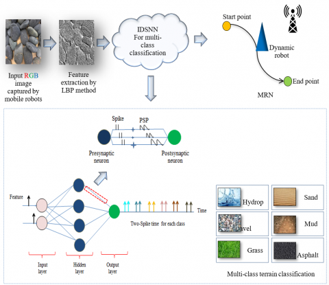
This section delineates the methodology employed in the proposed model for addressing the terrain classification challenge, with an emphasis on the integration of a SNN and vision-based techniques. The model, as depicted in Figure 1, comprises three distinct stages: feature extraction, classification, and subsequent application in MRN.
Figure 1. Terrain classification using the proposed model
3.1 Feature extraction stage
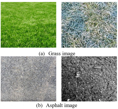
Initially, a dataset comprising 42,000 terrain images (each of size 256x256) across six terrain classes was collated (source: https://www.pinterest.com/dsfafsh/textures/). The feature extraction stage leverages the LBP method for extracting texture features from these images. The LBP method, noted for its simplicity, speed, and discriminative power [24, 25], was chosen due to the variability in terrain appearance throughout different seasons [26, 27]. For instance, Figure 2 illustrates variations in color for the same terrain type under different conditions; part (a) shows grass images in spring and winter, while part (b) contrasts dry and wet asphalt. Such variations in terrain appearance, influenced by factors like humidity, drought, and weather changes, significantly affect visual characteristics such as color. Reliance solely on color features could, therefore, lead to high misclassification rates. Consequently, the texture feature vector, consisting of 18 elements, is extracted as the output of this stage.
Figure 2. Terrain samples under different conditions
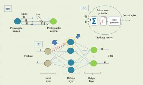
Figure 3. Structure of IDSNN
3.2 Classification stage
The classification stage is centered around the IDSNN, which serves as the classifier. Figure 3 illustrates the fully connected feed-forward structure of the IDSNN. This structure comprises three layers: the input layer, the hidden layer, and the output layer. The output layer consists of six neurons, each representing a terrain class (hydrop, gravel, grass, sand, mud, and asphalt) via a dual spike mechanism. The hidden layer contains 42 neurons, and the input layer encompasses six neurons corresponding to the texture feature vector. Each neuron in the SNN is characterized by multiple connections or synapses, each with varying delays and weights, as depicted in part (B) of Figure 3. The computational process within each neuron involves three steps: initially, the summation of all input spikes forms the membrane potential. Subsequently, it is assessed whether this potential exceeds a threshold value. If exceeded, the neuron emits a spike at time tf and the membrane potential is reset to zero, as detailed in part (C).
To facilitate classification, the methodology incorporates three main components: encoding and decoding functions, neuron model functions, and a modified learning method.
3.2.1 Encoding and decoding functions
In spiking neural networks, pulse information is dealt with instead of raw data. The initial stage of training involves the conversion of data into spike times using Eq. (1), where Tmax and Tmin denote the largest and smallest interval times, and Imax and Imin represent the maximum and minimum extracted feature values, respectively. Iin is the real value of the input data, and round is a function that rounds a number to specific digits.
$t_r^f=T_{\max }-{round}\left(T_{\min }+\frac{\left(I_{\text {in }}-I_{\min }\right)\left(T_{\max }-T_{\min }\right)}{I_{\max }-I_{\min }}\right)$ (1)
Post-training, the output spikes of each class are converted back to raw data using Eq. (2), wherein $O y\left(t_y^f\right)$ denotes the actual output spike time.
$O y\left(t_y^f\right)=\frac{\left(T_{\max }-t_y^f-T_{\min }\right) \times\left(I_{\max }-I_{\min }\right)}{\left(T_{\max }-T_{\min }\right)}+I_{\min }$ (2)
3.2.2 Neuron model function
Among the biologically plausible models used in spiking neural networks, such as the Spike Response Model (SRM), Izhikevich model, Hodgkin-Huxley (HH) model, and Integrate and Fire (IF) model [28], this paper utilizes the SRM due to its simplified mathematical approach [29]. The SRM's connection between input spikes and membrane potential is encapsulated in this model. In this study, the hyperbolic tangent function is employed in the SRM, as shown in Eq. (3), where ɛ(t) represents the spike response function, and τ is the time decay constant of ɛ.
$\varepsilon(t)=\left\{\begin{array}{c}0, t \leq 0 \\ \tanh (t / \tau), t>0\end{array}\right.$ (3)
The derivative of this function is presented in Eq. (4).
$\frac{\partial \varepsilon}{\partial t}=\frac{1}{\tau}\left(1-\tanh ^2(t / \tau)\right)$ (4)
3.2.3 Modified learning method
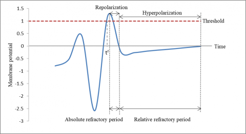
Upon encoding real data into spike times, the forward phase commences, starting from the hidden layer. In this phase, neurons are evaluated to determine whether they emit a spike. This occurs when the neuron's membrane potential surpasses a predefined threshold, at which point a spike is emitted at time tf, followed by the resetting of the membrane potential to zero. Post-spiking, the neuron undergoes two phases: repolarization and hyperpolarization. The former, known as the absolute refractory period, involves the membrane potential's decline to zero. The latter phase, the relative refractory period, is characterized by the membrane potential remaining below zero, making it more challenging for the neuron to emit a spike (Figure 4).
Figure 4. Absolute and relative refractory period phases
These phases are particularly pertinent in MSNNs, which deal with multiple spikes, as opposed to single-spike neural networks that handle only one spike time. Consequently, the refractoriness function, expressed in Eq. (5), is incorporated into the membrane potential calculation.
$\eta(t)=\left\{\begin{array}{c}-2 \times \vartheta \times \exp \left(-t / \tau_a\right), t>0 \\ 0, t \leq 0\end{array}\right.$ (5)
Eq. (5) considers the threshold value $\vartheta$ and the time decay constant τa. The membrane potential is computed based on the arrival time of input spikes after (trf + Rl), considering the most recent output spike time trf and the duration of the absolute refractory period Rl.
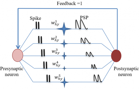
The general formula for the membrane potential of a spiking neuron in a multi-spike learning context, where neurons in adjacent layers are interconnected by multiple synapses s=1, 2, 3, ..., Sy, transmitting various spike times Fi=ti1, ti2, ti3, ..., tiFi from the presynaptic neuron (i) to the postsynaptic neuron (j), is shown in Eq. (6). This equation accounts for different delays ds and weights in the synaptic connections. The arrival spike time at neuron j is denoted as tif + ds. The equation of membrane potential mp(t) is shown below.
$m p(t)=\sum_{i=1}^{N_i} \sum_{s=1}^{S_y} \sum_{\substack{t_i^f \in F_i \\ t_i^f+d^s>t_j^{r f}+R_l}} w_{i j}^s \varepsilon\left(t-t_i^f-d^s\right)+\eta\left(t-t^{r f}\right)$ (6)
where, Ni is the index of presynaptic neurons, $w_{i j}^s$ is the weight of synapse between neurons i and j. Furthermore, the formula for the membrane potential of hidden neurons in the IDSNN model includes an additional term, reflecting the feedback from each output neuron to all hidden neurons, as shown in Eq. (7). This feedback mechanism, which comprises both current and previous outputs, enhances the model's memory and overall performance. Figure 5 depicts the sub-connection between two neurons with output feedback in the IDSNN model.
$O F B=\eta \sum_{o=1}^{N_o} \sum_{s=1}^{S_y} w_{h o}^s \times S_o(t-1)$ (7)
In the IDSNN model, several key parameters are integral to the functioning of the neural network. The learning rate, denoted by η, plays a crucial role in the network's training process. The number of output neurons, represented as NO, is a fundamental aspect of the network's architecture. Additionally, the weight of the synapse between the hidden and output layers, symbolized as $w_{h o}^s$, contributes significantly to the synaptic strength and information transmission within the network. Another critical element is So(t-1), which signifies the previous output of the output layer, serving as a feedback mechanism to the hidden neurons. Therefore, the membrane potential of the hidden neurons in the IDSNN model is formulated as per the following equation:
$m p_h(t)=\sum_{n=1}^{N_n} \sum_{s=1}^{S_y} \sum_{\substack{t_n^f \in F_n \\ t_n^f+d^s>t_h^{r f}+R_l}} w_{n h}^s \varepsilon\left(t-t_n^f-d^s\right)+\eta\left(t-t_h^{r f}\right)+$ OFB (8)
Eq. (8) illustrates the membrane potential of hidden neurons in the IDSNN model, factoring in the number of neurons Nn in the input layer and the synaptic weights $w_{n h}^s$ between input and hidden neurons.
The mean square error (MSE), represented in Eq. (9), serves as the error function, where $t_o^f$ indicates the actual output spike and $t_o^{f^{\prime}}$ represents the desired spike time for the output neuron (o). The number of output spikes Fo and the number of neurons in the output layer No are also considered.
$M S E=1 / 2 \sum_{o=1}^{N_o} \sum_{f=1}^{F_o}\left(t_o^f-t_o^{f^{\prime}}\right)^2$ (9)
Synaptic weights between neurons in the hidden and output layers are updated to minimize the error function, leveraging the gradient descent method. The computation of this update is outlined in Eqs. (10) and (11).
$w_{h o}^s(t+1)=w_{h o}^s(t)+\Delta w_{h o}^s(t)$ (10)
where,
$\Delta w_{h o}^S(t)=-\eta \nabla E_{h o}^s$ (11)
Similarly, the weights of synapses between neurons in the hidden and input layers are updated as per Eq. (12), with the computation detailed in Eq. (13).
$w_{n h}^s(t+1)=w_{n h}^s(t)+\Delta w_{n h}^s(t)$ (12)
where,
$\Delta w_{n h}^s(t)=-\eta \nabla E_{n h}^s$ (13)
Figure 5. Synapses of one connection with feedback in IDSNN model
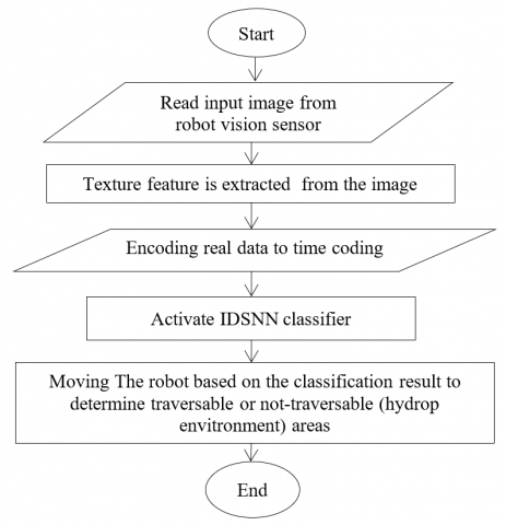
Figure 6. Flowchart of the proposed model
3.3 MRN
The IDSNN model is designed to enhance the outdoor navigation capabilities of UGVs. This process involves a sequence of three steps for environment identification and subsequent navigation. In the initial step, terrain images are captured by the UGV utilizing vision sensors, such as a Point-Grey Firefly color camera with a resolution of 640×480, positioned 50cm above the ground. Images are acquired starting from a 30cm distance. Following this, the features are extracted from the captured images. The second step entails the input of the extracted feature vector into the trained IDSNN model to determine the upcoming terrain type. This identification is crucial for the subsequent navigation strategy of the UGV. The final step involves the actual navigation of the UGV. Special attention is given to hydrop terrain, identified as particularly hazardous due to its potential to cause damage to the robot. In scenarios where the classified terrain is hydrop, the UGV is programmed not to proceed. Conversely, if the terrain is classified as any type other than hydrop, commands are sent to the on-board motors to facilitate movement.
The operational flow of the proposed model is summarized in a flowchart, depicted in Figure 6.
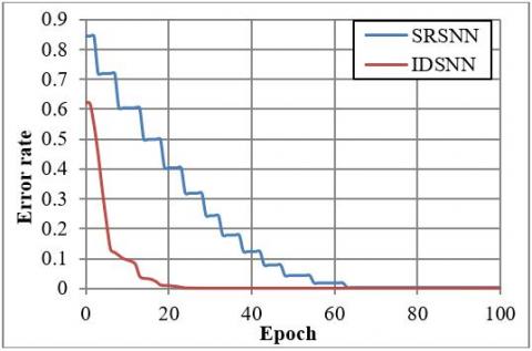
The implementation of the IDSNN was conducted using the Spyder simulator on a DELL laptop, featuring a Windows 10 operating system and an Intel CORE i5 CPU. Python language was utilized for programming purposes. The dataset gathered for this study was divided into two segments: 70% allocated for the training set and 30% for the testing set. The neuronal parameters of the IDSNN are detailed in Table 1. Synaptic connections between pairs of neurons were characterized by five synapses, each having distinct delays of 1, 5, 9, 13, and 17 milliseconds. The IDSNN model's performance was evaluated using key metrics such as accuracy, precision, recall, and F1-score. A comparative analysis between the IDSNN and the SRSNN, which shares a similar structure with the IDSNN, was undertaken to ensure a fair comparison. Figure 7 depicts the error rates of both models across various epochs, illustrating a faster decrease in error rate for the IDSNN (represented by a red line) compared to the SRSNN (blue line). This is evident from the IDSNN's initial error rate of 0.62 decreasing rapidly, reaching the error goal by the 22nd epoch, whereas the SRSNN starts at an error rate of 0.85 and achieves the error goal around the 63rd epoch. This data underscores the IDSNN's enhanced accuracy and more rapid learning capability, attributable to the efficacy of its multi-spike structure, which improves classification reliability.
Figure 7. Error rate of IDSNN vs. SRSNN
Accuracy $=\frac{T P+T N}{T P+T N+F P+F N} * 100 \%$ (14)
Precision $=\frac{T P}{T P+F P} * 100 \%$ (15)
Recall= $=\frac{T P}{T P+F N} * 100 \%$ (16)
F1-score $=\frac{(2 * \text { Recall } * \text { Precision })}{\text { Precision }+ \text { Recall }}$ (17)
Table 1. Neuron parameters in IDSNN
|
Parameters |
Values |
|
τ |
11ms |
|
Rl |
1ms |
|
τr |
80 ms |
|
ϑ |
1v |
|
η |
0.001 |
Table 2. Overall performance of IDSNN vs. SRSNN
|
Metrics |
SRSNN |
IDSNN |
|
Accuracy |
87.222% |
90.706% |
|
Precision |
87.310% |
90.768% |
|
Recall |
87.231% |
90.715% |
|
F1-score |
87.270 |
90.741 |
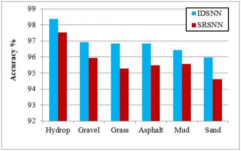
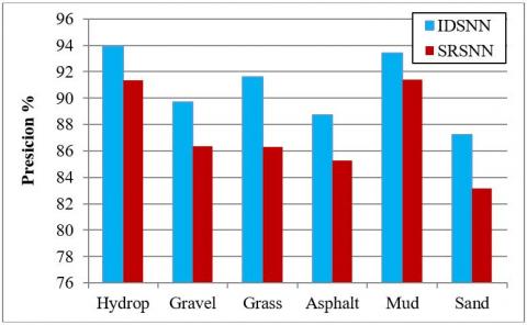
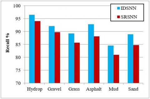
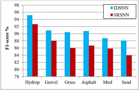
In the IDSNN evaluation, standard classification metrics were employed. True Positives (TP) represents the count of samples correctly classified as belonging to the positive class, while True Negative (TN) denotes the count of samples accurately identified as belonging to the negative class. Conversely, False Positive (FP) exemplifies instances where negative class samples are incorrectly classified as positive, and false negative (FN) indicates misclassification of positive class samples. Figure 8 presents a comparison of the accuracy for each terrain class between the multi-spike learning approach of IDSNN and the single-spike learning of SRSNN. It is observed that the IDSNN model exhibits higher accuracy, attributable to the enhanced reliability of classification fostered by the multi-spike learning mechanism, where double spikes represent each class. The precision ratio of IDSNN, in comparison to SRSNN, is illustrated in Figure 9. A higher precision ratio in IDSNN indicates a lower frequency of false positive predictions and a higher occurrence of true positives, signifying enhanced model precision. In the context of recall, which is critically important for identifying hazardous terrains such as hydrop, IDSNN surpasses SRSNN in recall ratio, as depicted in Figure 10. This indicates that IDSNN is more effective in minimizing misclassifications, especially in critical terrain types. Furthermore, the F1-score, which reflects the balance between precision and recall, is employed to assess the overall efficacy of the models. A higher F1-score suggests a harmonious balance between precision and recall within the model. As shown in Figure 11, the F1-score for IDSNN is superior to that of SRSNN, indicating that IDSNN is more efficient in its classification capabilities.
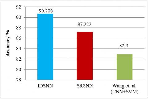
The overall accuracy of the proposed two models is compared with the overall accuracy of Wang et al. [6], where the IDSNN model and SRSNN model achieve better performance in accuracy compared to Wang et al. [6], as shown in Figure 12. This is because the intelligent structure of the proposed two models contains feedback from the output layer to the hidden layer. With feedback, the input includes the previous output and the present input. Hence, the memory of the model will be enhanced. Thus, enhancing the performance of the model and making the model more accurate. Additionally, the SNN deals with spike time, unlike the traditional neural network which deals with real data. Moreover, the IDSNN model achieves better performance in accuracy compared to SRSNN model. This is because dealing with double spikes can be more robust to noise and variations in the input data compared to SRSNN that made the IDSNN more accurate.
Figure 8. Accuracy values of IDSNN vs. SRSNN
Figure 9. Precision values of IDSNN vs. SRSNN
Figure 10. Recall values of IDSNN vs. SRSNN
Figure 11. F1-score values of IDSNN vs. SRSNN
Figure 12. The overall accuracy of IDSNN vs. SRSNN and Wang et al. [6]
Table 1 lists the neuron parameters used in the IDSNN model, while Table 2 presents a comprehensive comparison of the overall performance between IDSNN and SRSNN. It is evident that IDSNN outperforms SRSNN by approximately 3%.
A potential limitation of this study is the selection of the spiking neural network structure, which was determined through trial and error. Future research could explore the application of a fuzzy logic controller to optimize the parameters of the SNN, potentially enhancing the model's efficiency and accuracy.
The IDSNN has been proposed as a solution to the terrain classification challenge, leveraging the advantages of multi-spike learning with temporal coding. This model successfully determines six types of terrains (hydrop, gravel, grass, sand, mud, and asphalt) based on texture features. When compared with the SRSNN using metrics such as accuracy, precision, recall, and F1-score, the IDSNN model demonstrates superior performance.
The simulation results lead to several key conclusions:
·The IDSNN model exhibits a more robust capability than the SRSNN model. This superiority is attributed to the limitations of single-spike learning in handling finite information, a constraint effectively overcome by multi-spike learning.
·IDSNN's accuracy and learning speed surpass that of SRSNN, owing to the enhanced reliability of classification provided by multi-spike learning.
·In terms of classification performance for all six terrain types, especially in hazardous terrains such as hydrop, the IDSNN model shows significant advancements over the SRSNN model.
·The IDSNN model effectively assists UGVs in outdoor navigation by accurately identifying areas as traversable or untraversable, thus enabling optimal decision-making for movement.
Suggestions for future work:
·Further enhancement of the proposed model can be achieved by integrating a fusion of visual and geometric features, instead of relying solely on visual features.
·Development of a more intelligent terrain classification controller is recommended, particularly for classifying mixed terrain.
[1] Atiyah, H.A., Hassan, M.Y. (2023). Outdoor localization for a mobile robot under different weather conditions using a deep learning algorithm. Journal Européen des Systèmes Automatisés, 56(1): 1-9. https://doi.org/10.18280/jesa.560101
[2] Jawad, M.M., Hadi, E.A. (2019). A comparative study of various intelligent algorithms based path planning for mobile robots. Journal of Engineering, 25(6): 83-100. https://doi.org/10.31026/j.eng.2019.06.07
[3] Al-Araji, A.S., Ahmed, A.K., Dagher, K.E. (2019). A cognition path planning with a nonlinear controller design for wheeled mobile robot based on an intelligent algorithm. Journal of Engineering, 25(1): 64-83. https://doi.org/10.31026/j.eng.2019.01.06
[4] Zou, X., Hwu, T., Krichmar, J., Neftci, E. (2020). Terrain classification with a reservoir-based network of spiking neurons. In 2020 IEEE International Symposium on Circuits and Systems (ISCAS), Seville, Spain, pp. 1-5. https://doi.org/10.1109/ISCAS45731.2020.9180740
[5] Yu, Z., Sadati, S.H., Wegiriya, H., Childs, P., Nanayakkara, T. (2021). A method to use nonlinear dynamics in a whisker sensor for terrain identification by mobile robots. In 2021 IEEE/RSJ International Conference on Intelligent Robots and Systems (IROS), Prague, Czech Republic, pp. 8437-8443. https://doi.org/10.1109/IROS51168.2021.9636571
[6] Wang, W., Zhang, B., Wu, K., Chepinskiy, S.A., Zhilenkov, A.A., Chernyi, S., Krasnov, A.Y. (2022). A visual terrain classification method for mobile robots’ navigation based on convolutional neural network and support vector machine. Transactions of the Institute of Measurement and Control, 44(4): 744-753. https://doi.org/10.1177/0142331220987917
[7] Hanson, N., Shaham, M., Erdoğmuş, D., Padir, T. (2022). Vast: Visual and spectral terrain classification in unstructured multi-class environments. In 2022 IEEE/RSJ International Conference on Intelligent Robots and Systems (IROS), Kyoto, Japan, pp. 3956-3963. https://doi.org/10.1109/IROS47612.2022.9982078
[8] Papadakis, P. (2013). Terrain traversability analysis methods for UGVs: A survey. Engineering Applications of Artificial Intelligence, 26(4): 1373-1385. https://doi.org/10.1016/j.engappai.2013.01.006
[9] Schilling, F., Chen, X., Folkesson, J., Jensfelt, P. (2017). Geometric and visual terrain classification for autonomous mobile navigation. In 2017 IEEE/RSJ International Conference on Intelligent Robots and Systems (IROS), Vancouver, BC, Canada, pp. 2678-2684. https://doi.org/10.1109/IROS.2017.8206092
[10] Zou, Y., Chen, W., Xie, L., Wu, X. (2014). Comparison of different approaches to visual terrain classification for outdoor mobile robots. Pattern Recognition Letters, 38: 54-62. https://doi.org/10.1016/j.patrec.2013.11.004
[11] DuPont, E.M., Moore, C.A., Roberts, R.G. (2008). Terrain classification for mobile robots traveling at various speeds: An eigenspace manifold approach. In 2008 IEEE International Conference on Robotics and Automation, Pasadena, CA, USA, pp. 3284-3289. https://doi.org/10.1109/ROBOT.2008.4543711
[12] Ran, T., Yuan, L., Zhang, J.B. (2021). Scene perception based visual navigation of mobile robot in indoor environment. ISA Transactions, 109: 389-400. https://doi.org/10.1016/j.isatra.2020.10.023
[13] Ruan, X., Ren, D., Zhu, X., Huang, J. (2019). MRN based on deep reinforcement learning. In 2019 Chinese Control and Decision Conference (CCDC), Nanchang, China, pp. 6174-6178. https://doi.org/10.1109/CCDC.2019.8832393
[14] Zarzoor, A.R., Al-Jamali, N.A.S., Al-Saedi, I.R. (2023). Traffic classification of IoT devices by utilizing spike neural network learning approach. Mathematical Modelling of Engineering Problems, 10(2): 639-646. https://doi.org/10.18280/mmep.100234
[15] Shiltagh, N.A., Abas, H.A. (2015). Spiking neural network in precision agriculture. Journal of Engineering, 21(7): 17-34. https://doi.org/10.31026/j.eng.2015.07.02
[16] Xu, Y., Zeng, X., Han, L., Yang, J. (2013). A supervised multi-spike learning algorithm based on gradient descent for spiking neural networks. Neural Networks, 43: 99-113. https://doi.org/10.1016/j.neunet.2013.02.003
[17] Taherkhani, A., Belatreche, A., Li, Y., Maguire, L.P. (2018). A supervised learning algorithm for learning precise timing of multiple spikes in multilayer spiking neural networks. IEEE Transactions on Neural Networks and Learning Systems, 29(11): 5394-5407. https://doi.org/10.1109/TNNLS.2018.2797801
[18] Aljamali, N.A.S. (2020). Convolutional multi-spike neural network as intelligent system prediction for control systems. Journal of Engineering, 26(11): 184-194. https://doi.org/10.31026/j.eng.2020.11.12
[19] Yu, Z., Sadati, S.H., Hauser, H., Childs, P.R., Nanayakkara, T. (2022). A semi-supervised reservoir computing system based on tapered whisker for mobile robot terrain identification and roughness estimation. IEEE Robotics and Automation Letters, 7(2): 5655-5662. https://doi.org/10.1109/LRA.2022.3159859
[20] Wang, M., Ye, L., Sun, X. (2021). Adaptive online terrain classification method for mobile robot based on vibration signals. International Journal of Advanced Robotic Systems, 18(6): 17298814211062035. https://doi.org/10.1177/17298814211062035
[21] Yang, H., Jie, W., Qian, N. (2020). A new terrain classification algorithm based on convolutional neural network. In 2020 International Conference on Information Science, Parallel and Distributed Systems (ISPDS), Xi'an, China, pp. 313-317. https://doi.org/10.1109/ISPDS51347.2020.00072
[22] Chen, Y., Rastogi, C., Norris, W.R. (2021). A CNN based vision-proprioception fusion method for robust UGV terrain classification. IEEE Robotics and Automation Letters, 6(4): 7965-7972. https://doi.org/10.1109/LRA.2021.3101866
[23] Soud, N.S., Al-Jamali, N.A.S., Al-Raweshidy, H.S. (2022). Moderately multispike return neural network for SDN accurate traffic awareness in effective 5G network slicing. IEEE Access, 10: 73378-73387. https://doi.org/10.1109/ACCESS.2022.3189354
[24] Singh, C., Walia, E., Kaur, K.P. (2018). Color texture description with novel local binary patterns for effective image retrieval. Pattern Recognition, 76: 50-68. https://doi.org/10.1016/j.patcog.2017.10.021
[25] Karis, M.S., Razif, N.R.A., Ali, N.M., Rosli, M.A., Aras, M.S.M., Ghazaly, M.M. (2016). Local binary pattern (LBP) with application to variant object detection: A survey and method. In 2016 IEEE 12th International Colloquium on Signal Processing & Its Applications (CSPA), Melaka, Malaysia, pp. 221-226. https://doi.org/10.1109/CSPA.2016.7515835
[26] Khan, Y.N., Komma, P., Zell, A. (2011). High resolution visual terrain classification for outdoor robots. In 2011 IEEE International Conference on Computer Vision Workshops (ICCV Workshops), Barcelona, Spain, pp. 1014-1021. https://doi.org/10.1109/ICCVW.2011.6130362
[27] Zürn, J., Burgard, W., Valada, A. (2020). Self-supervised visual terrain classification from unsupervised acoustic feature learning. IEEE Transactions on Robotics, 37(2): 466-481. https://doi.org/10.1109/TRO.2020.3031214
[28] Yellakuor, B.E., Moses, A.A., Zhen, Q., Olaosebikan, O.E., Qin, Z. (2020). A multi-spiking neural network learning model for data classification. IEEE Access, 8: 72360-72371. https://doi.org/10.1109/ACCESS.2020.2985257
[29] Oniz, Y., Kaynak, O., Abiyev, R. (2013). Spiking neural networks for the control of a servo system. In 2013 IEEE International Conference on Mechatronics (ICM), Vicenza, Italy, pp. 94-98. https://doi.org/10.1109/ICMECH.2013.6518517