Optimisation of Supply Chain with Reactive Lateral Transhipment Under Imperfect Production System

Batik, is one of the leading products by Indonesia and has extensive use on the domestic market and high value on the international market. Therefore, enhancing the supply chain system for batik products will have long-term benefits. A crucial decision in the batik supply chain system is the strategy for ordering products from buyers to vendor, which affects the production management at the vendor. This strategy decision will have an effect on the demand fulfilment that can be converting into competitive advantage and profitability to the entire supply chain. Several previous researchers have paid attention to this topic because it is significant and strategic with different conditions, such as multiple shipment policy [1], time-phased price discount [2] and price-sensitive demand [3].

Obviously, each buyer in the batik supply chain will receive random customer demand. However, after a period of time, the demand pattern can be modelled with a statistical distribution, which is preferable to the average value [4]. This study will also model users demand using statistical distributions approach. In addition, it is common for products to be shipped from one buyer to another because shipping costs are comparatively low and the response time is fast, despite the fact that the purchase price of the product is higher than purchase price from the vendor. This is referred to as lateral transhipment in the distribution system [5], that typically aimed to balance the inventory level of the chains at the same echelon [6]. In contrast to the typical lateral transhipment system, in the investigated supply chain system, product delivery from one buyer to another will occur only upon request; this is comparable to reactive literal transhipment [7].

The buyers often adopt a minimum inventory policy when faced with uncertain demand, taking into account the lead time for orders from vendors and other buyers.  On the vendor side, the vendor will control the daily Economic Production Quantity (EPQ) because customer demands do not arrive simultaneously. The EPQ will be determined by considering optimum utilisation of the vendor production resources [8, 9].

Production process of batik is usually semi-automatic. The batik printers are controlled by operators. At the beginning, the operators will setup the batik printers and after several production units, defective products will occur, necessitating a setup of the batik printers. Such a production system is called an imperfect production system [10, 11]. The defective batik products will be reworked, but not all will be repairable. If a batik product cannot be repaired, it will be converted into patchwork. Consequently, the EPQ in the imperfect production system will be determined by considering the occurrence of defective products and the rework process. In this situation, the problem will grow intricate because of the numerous variables involved, and it will be further compounded when multiple products must be produced.

The majority of problem-solving optimisation algorithms utilise static data. When the number of decision variables is small, the exact optimisation algorithm can generate the optimum solution in a reasonable computation time. However, if the number of decision variables is very large, the resulting solution is only a feasible one, with no guarantee of optimality or one that is near to optimum. Genetic Algorithms (GA), which was coined by John Holland, can be utilised as an optimisation algorithm for stochastic models with a large number of decision variables [12]. Therefore, in this study, GA will be used as the optimisation algorithms, and since the demands data are modelled using statistical distribution and the information and materials flow are flowing dynamically in the supply chain system, then the GA will be used in-the-loop with the supply chain simulation system. This technique has several different terms, such as simulation optimisation [13] and optimisation-simulation closed-loop [14]. In this study, this technique will be called as optimisation-in-the-loop simulation. The previous studies shown that advantage of optimisation-in-the-loop simulation technique is the optimisation algorithm received dynamic feedbacks from the simulation during optimisation process so that the solution provided is the best solution in the steady state condition. This advantage is also used to address optimisation problem in the present study.

3.1 The supply chain description

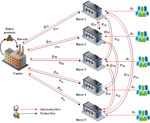
The supply chain system under consideration has one vendor and five buyers. There are five batik products that flow across the supply chains. The historical data indicates that Buyer 2 and 3 sometime make purchases from Buyer 1. On the other side, Buyers 1 and 3 sometime place an order to Buyer 5, whereas Buyer 4 sometime orders from Buyer 2. Lateral transhipment refers to the practice of one buyer utilising another buyer's on-hand inventory. When the buyers anticipate stock-outs and place orders to other buyers, this is referred to as reactive transhipment [34]. Figure 1 depicts the supply chain system diagram under consideration.

As described in the introduction, after several production units, the semi-automatic batik printers occasionally produce prints with defects. However, not all batik with printing defects can be reworked into successful batik goods. In order for vendors to fulfil orders from all customers, the production quantity of the batik products must take into account the probability that the batik printers will produce defective products and the number of defective batik products that can be reworked.

3.2 The supply chain system variables and parameters

The supply chain system was simulated using Microsoft Excel, during the simulation, the decision variables were optimised using GA. Therefore, this case study is considered as simulation-based stochastic optimisation. The decision variables and the parameters are explained in the nomenclature section at the end of this paper.

1.png

Figure 1. The supply chain system diagram under consideration

3.3 Mathematical models development

The main objective of the optimisation model is to minimise JTC, which consists of VTC and BTC. The subsequent sections detail the model development procedure.

3.3.1 VTC model

The first cost element of the VTC is VSC, determined by multiplying the total number of production runs for all products by the setup cost per production run for all products. The following formula represents the VSC formula.

$V S C=\sum_{p=1}^P \sum_{t=1}^T S_{p t} \times P R_{p t}$

$P R_{p t}=\left\{\begin{array}{l}1, \text { if } P D_p>0 \\ 0, \text { otherwise }\end{array}\right.$      (1)

The second cost element of the VTC is VLC, determined by multiplying the total number of lost sales for all products by the lost sales cost per unit for all products. The following formula expressed the VLC formula.

$V L C=\sum_{p=1}^P \sum_{t=1}^T L S_{p t} \times L O_{p t}$

$L O_{p t}=\max \left(0 ; D_{p t}-\left(P D_{p t}+P_{p t-1}\right)\right)$

$D_{p t}=\sum_{b=1}^B Q_{p t b} ; \forall p ; \forall t$     (2)

The next cost element of the VTC is VHC, determined by multiplying total ending inventories of all products by their carrying costs. The equation below illustrates the VHC formula.

$V H C=\sum_{p=1}^P \sum_{t=1}^T H_{p t} \times I_{p t}$

$I_{p t}=\max \left(0 ;\left(P D_{p t}+P_{p t-1}\right)-D_{p t}\right)$

$D_{p t}=\sum_{b=1}^B Q_{p t b} ; \forall p ; \forall t$     (3)

The last component of the VTC is the VWC, determined by multiplying the number of reworked all products by their rework costs per unit. The following equation depicts the VWC formula.

$V W C=\sum_{p=1}^P \sum_{t=1}^T P D_{p t} \times p o_{p t} \times R W_p$

$p o_{p t}=\left\{\begin{array}{c}0 \leq p o_{p t} \leq P O_p, \text { if } \sum_{0,} P D_p \geq w_p \\ 0, \quad \text { otherwise }\end{array}\right.$     (4)

Hence, the VTC can be expressed as indicated by the following formula.

$V T C=V S C+V L C+V H C+V W C$     (5)

3.3.2 BTC model

The BTC consists of BOC, BLC, and BHC. The BOC is determined by multiplying the order frequency during simulation by the ordering cost to the vendor or another buyer, as indicated in the following formula.

$B O C=\sum_{a=1}^B \sum_{b=1}^B \sum_{p=1}^P \sum_{t=1}^T\left(\left(A_{0 t} \times n o_{p a 0 t}\right)+\left(A_{a b t} \times n o_{p a b t}\right)\right) ; a \neq b$

$n o_{\text {pa0t }}=\left\{\begin{array}{c}1, \text { if } Q_{p a 0}>0 \\ 0, \text { otherwise }\end{array}\right.$

$n o_{\text {pabt }}=\left\{\begin{array}{c}1, \text { if } Q_{\text {pab }}>0 \\ 0, \text { otherwise }\end{array}\right.$     (6)

The BLC is calculated by multiplying the cost of lost sales for all products by the total number of lost sales for all products across all buyers, as indicated in the following equation.

$B L C=\sum_{b=1}^B \sum_{p=1}^P \sum_{t=1}^T l s_{b p t} \times l o_{b p t}$

$l o_{b p t}=\max \left(0 ; d_{b p t}-\left(Q_{p a 0}+Q_{p a b}+i_{p t-1}\right)\right)$     (7)

The BHC is calculated by multiplying the carrying cost for all products by the number of ending inventories for all products across all buyers, as stated in the following equation.

$B H C=\sum_{b=1}^B \sum_{p=1}^P \sum_{t=1}^T h_{b p t} \times i_{b p t}$

$i_{b p t}=\max \left(0 ;\left(Q_{p a 0}+Q_{p a b}+i_{p t-1}\right)-d_{b p t}\right)$      (8)

To calculate the BTC, sum the values of BOC, BLC, and BHC, as depicted in the following equation.

$B T C=B O C+B L C+B H C$      (9)

3.3.3 JTC model

The JTC, which is the sum of the VTC and BTC, indicates the entire cost of the supply chain system, as indicated in the following formula.

$J T C=V T C+B T C$     (10)

3.4 GA development

As an optimisation tool, there are three essential components of genetic algorithms that are chromosome development, fitness function determination, and genetic operations including crossover and mutation. In the subsequent sub-sections, all of these essential details will be elaborated.

3.4.1 Chromosome model

As an evolutionary optimisation algorithm, GA will encode a model's decision variables as chromosomes to determine their optimal value. Table 1 displays the decision variable of the supply chain optimisation model and how they are encoded in the proposed GA. The decision variables are constrained to a maximum value of 3000 units due to the production capacity of the vendor and the overall buyer's demand, which never surpasses 3000 units. In order to provide a wide range of values for a gene by using a sufficient number of bits, therefore binary encoding is used in the proposed GA.

When a is the index for all buyers and b is the index for buyer that received order from another buyer, according to Figure 1, then a will move from 1 to 5 and b value will be 1, 2 and 5. Therefore, there will be P×5×5 genes in a chromosome. The proposed GA will be integrated with the supply chain simulation, resulting in a substantial increase in computation time. In order to reduce the computation time, the population size is made variable. The initial population size is fixed, and in subsequent generations, identical chromosomes will be reduced to two copies only, resulting in a decrease in population size. It will also prevent the GA from being stuck in local optimal conditions caused by the dominance of super chromosomes.

Table 1. The decision variables and their encoding

3.4.2 Fitness function determination

In GA, chromosomes with a high fitness value are able to survive until the final generation; thus, it is associated with maximisation. However, the objective of this study's optimisation model is to minimise the JTC, which is contrary to the GA searching concept. Therefore, fitness function of the chromosome is formulated as a big number, that always higher than JTC, subtracted by average of JTC during simulation, as shown in Eq. (11).

$e v=g-\frac{J T C}{T}$     (11)

3.4.3 Crossover mechanism

This study employs a standard one-cut point crossover, which is based on randomly defined cutting points and normal sub-gene exchange. Nevertheless, the crossover operation is carried out for each gene on a chromosome. The mechanism of the one-cut point crossover for each gene is depicted in Figure 2.

2.png

Figure 2. Mechanism of the one-cut point crossover

3.4.4 Mutation mechanism

A semi-guided non-uniform mutation process is utilised in the GA to explore values inside a variable's current value and its limit value. This mutation process alters the traditional non-uniform mutation method introduced by Michalewicz [12]. The modification aims to increase the efficiency of the GA's exploration while preserving the stochastic character of its process. The mutation method directs the GA to adjust the mutant gene based on its fitness value. Despite this, the change in value remains arbitrary. The method of the semi-guided non-uniform mutation is explained by following procedure.

Step 1: Select a gene in a chromosome based on mutation probability;

Step 2: Decode the gene to be integer value;

Step 3: Increase the decoded value with random delta and still lower than or equals to the maximum limit;

Step 4: Evaluate the fitness value, if the fitness value is better than current fitness value, then go to Step 6, otherwise go to Step 5;

Step 5: Decrease the decoded value with random delta and still higher than or equals to the minimum limit;

Step 6: Encode the gene.

For example, a randomly selected gene for PD₁ 00011101 is converted to the value 29 by the decoding step. The next step will increase this value at random to 35. If the JTC with the new PD₁ value is superior to the JTC with the previous PD₁ value, the new PD₁ value will be encoded and reinserted into the chromosome. If not, the previous PD₁ value is reduced, encoded, and reinserted into the chromosome.

From the preceding explanation, it can be concluded that the proposed optimisation model is able to provide optimum solution for the batik supply chain system under consideration, as indicated by the convergent GA. The proposed optimisation-in-the-loop simulation model is also capable of providing optimum solutions under steady-state conditions. From a managerial standpoint, the solutions are more reliable when dealing with changes in situations that do not change considerably. Another managerial recommendation is controlling the stock at the buyers from time to time to avoid lost sales. However, inventory level at the vendor is relatively stable. One of the most difficult aspects of using GA is ensuring that the algorithm does not become stuck in local optimum due to premature convergence and that it provides local optimum solutions. Because the proposed GA does not experience premature convergence, then the GA used in the optimisation-in-the-loop simulation system can be said fairly able to provide optimum solutions.

For subsequent research, when the out-of-control probability of the vendor production system becomes high, the vendor requires a high level of autonomy to manage production planning and inventory control. The optimisation model for chain systems should be modified to a vendor-managed inventory (VMI) model. With the aid of information technology, the VMI model's optimisation results will be readily implemented with a high level of demand satisfaction at the buyers.