Ali H. Alwan*![]() | Suhad A. Ali
| Suhad A. Ali![]() | Ashwaq T. Hashim
| Ashwaq T. Hashim![]()
© 2024 The authors. This article is published by IIETA and is licensed under the CC BY 4.0 license (http://creativecommons.org/licenses/by/4.0/).
OPEN ACCESS
Medical image segmentation is a crucial task in the field of medical imaging, and deep learning models have exhibited exceptional performance in recent years for segmentation purposes. In this paper, a refined network architecture of U-Net has been proposed, wherein residual units are included in U-Net to enhance the effectiveness of brain tumor segmentation. It constructs a deep learning model for the specific magnetic resonance imaging (MRI) segmentation task using the BraTS2020 dataset. The proposed enhanced model is designed by adding inner skip layers (residual connections) with fewer convolution layers to Allow the network to acquire knowledge of the residual mapping refers to the relationship between inputs layers and outputs layers instead of the direct mapping, consequently increasing the intersection over union (IoU). The results showed that after 100 epochs of training, the IoU of the proposed enhanced model is 0.910, while the model's accuracy is 0.968. In comparison, the original U-Net model achieved an Intersection over Union (IoU) score of 0.746 and an accuracy of 0.988 after 100 epochs. A comparison study was conducted with state-of-the-art work to demonstrate the effectiveness of the proposed enhancement in improving the performance of deep learning models for MRI segmentation. The promising results clearly indicate the potential of this enhancement.
medical imaging, magnetic resonance imaging, deep learning, U-Net, residual U-Net, segmentation, brain tumour
Medical image MRI (magnetic resonance imaging) is a potent diagnostic technology employed by health-care professionals to visualize the inside structures of the body [1]. The process involves the usage of radio waves, potent magnetic field, and computer technology to generate detailed images of bodily parts, tissues, and bones. MRI can produce high-quality, three-dimensional images of the body, making it an essential tool for diagnosing and treating various medical conditions, such as brain and spinal cord damage, cancer, and cardiovascular disease. MRI technology is non-invasive and employs harmless radiation, makes it a safe than others imaging techniques like X-rays and CT scans [2]. MRI scanners come in different sizes and designs, ranging from large machines used in hospitals to smaller, portable devices used in clinics or ambulances. The type of MRI used will depend on the specific needs of the patient and the medical condition being diagnosed. Overall, medical image MRI is a valuable tool in modern healthcare that helps healthcare professionals accurately diagnose and treat medical conditions, leading to better patient outcomes [3].
MRI scans can diagnose and characterize brain tumors [4]. Here are some of the most common ones: T1-weighted MRI: This type of MRI provides excellent detail of the brain's anatomy and can be used to identify tumors based on their location and size. Tumors appear as dark or bright spots on the image. T2-weighted MRI: This type of MRI is used to visualize the water content in tissues and can help identify areas of swelling and inflammation associated with tumors. Tumors appear as areas of increased brightness on the image. FLAIR MRI abbreviation for fluid-attenuated inversion recovery magnetic resonance imaging: This type of MRI is similar to a T2-weighted MRI but is designed to suppress the signal from cerebrospinal fluid (CSF) so that abnormalities in the brain are more visible. Tumors appear as bright areas on the image [5]. Diffusion-weighted MRI: This type of MRI is used to visualize the movement of water molecules in tissues and can help differentiate between different types of tumors. Tumors appear as areas of restricted diffusion on the image. Perfusion MRI: This type of MRI measures the flow of blood in the brain and can help identify areas of increased blood flow associated with tumors. Brain segment in magnetic resonance imaging MR is a crucial component of image analysis system, because it allows for the precise measurement of the volume of various brain structures and gives additional information to aid in the detection and quantification of lesions. Brain segmentation has various clinical applications, including assessing brain atrophy, identifying multiple sclerosis (MS) lesions, studying progress of brain development in various ages and image guided surgery [6-9]. In last years, deep learning has become One of the best areas for image segmentation, mainly using convolutional neural networks (CNNs). Overall, the U-Net and its variations have become a popular choice for image segmentation in many fields, including biomedical imaging and robotics, and research on the U-Net and its variations continues to be active [10]. Image segmentation using deep learning is an effective tool for extracting features from digital images. (CNNs), in recent years have become the go-to approach for image segmentation tasks. The U-Net architecture is widely recognized as one of the well-known CNN architectures for image segmentation, it relies on the concept of encoder-decoder. Before the advent of U-Net, segmentation tasks typically relied on the "sliding window" approach, where each pixel's class label was predicted by considering it as the center of a sliding window (patch). However, this method had several shortcomings that hindered its efficiency. Firstly, the time consumed by the sliding window to scan the entire image was considerable, making it computationally expensive. Additionally, the overlapping between patches caused redundancy in processing, leading to inefficiencies. Another challenge was finding the optimal patch size, as it required striking a balance between spatial localization accuracy and the effective utilization of contextual information. These limitations prompted the need for more efficient and accurate segmentation methods like the U-Net architecture [11].
The U-Net applies sequences of convolutional layers in the encoder to capture characteristics (features) of an input image and then uses a series of deconvolutional layers in the decoder to reconstruct the segmented image. Since its inception in 2015, the U-Net has been used in numerous applications, ranging from medical imaging to object detection [4]. It measures the similarity of the predicted mask and the ground truth mask by calculating the intersection area between the two masks divided by their union area. IoU (Intersection Over Union) score used to evaluation metric in computer vision and image segmentation tasks [12]. It evaluates the degree of similarity of two data sets, such as truth segment prediction. The IoU score is calculated by calculating the intersection area between the predicted and ground regions truth segmentation maps by the area of their union. The result is a value is 0 or 1, the score of 1 indicating complete overlap between the data sets. The IoU score is often used to evaluate the accuracy of object detection and segmentation models in computer vision applications, such as medical image analysis or autonomous driving. It is a reliable metric that can provide insights into the quality of the model's predictions. It can compare different models or fine-tune model parameters for better performance. In summary, the IoU score is a simple and effective measure of the similarity of two sets of data, and it is widely used in computer vision tasks to evaluate the metrices of segmentation models.
In light of the above, and due to the importance of automated brain tumor segmentation due to the complexity and time-consuming nature of manual diagnosis using MRI images, this work presents a new proposed deep learning network structure that apply residual U-Net by adding a skip layer to connect the layers of convolutions to maximums feature extraction in aims of increase the IoU due to the significant role of the more accurate resultant segmented image in obtaining the most ROI for medical imaging [13].
Medical image segmentation is considered an important topic that contributes as a fundamental step in many applications in the medical field and other related fields. The process of extracting a part of the image and working on it is a practical step in focusing on the critical part needed by a specific application instead of working on the entire image. One of these applications is the diagnosis of tumors and brain-related diseases. Therefore, this topic has become a recent trend for many researchers, and work on this topic is still under development, as there are constantly evolving segmentation algorithms. These studies aim to obtain efficient models with the highest standards and the lowest cost possible. With the continuous advancement of medical imaging technology, the need for accurate and efficient segmentation techniques is growing, and researchers are working on improving the performance and accuracy of these techniques.
Furthermore, the development of these techniques can significantly improve patient care and diagnosis accuracy, highlighting the importance of this field and the need for further research and development. Numerous studies have been reviewed in medical image segmentation using U-Net, and the strengths and weaknesses of the proposed methods by researchers, particularly those working with residual technology, have been discussed. The IoU factor for identifying brain tumor regions in medical images has also been discussed.
Aghalari et al. [14] improved U-Net -based architectures for automatic localization of brain tumors from MRI images were produced to solve the Glioma, a challenging brain tumor to diagnose due to its shape is not symmetrical and its borders appear blurry. The modified U-Net architecture incorporates both local and global features concurrently while reducing the parameters numbers compared to the original U-Net. Hence, they were evaluated on the BRATS'2018 database and achieved good results with lower calculation costs. The best-proposed model achieved Dice coefficient score "DCS", sensitivity, and positive predictive value PPV criteria values of 89.76%, 89.19%, and 90.65% for segmentation results.
Xiao et al. [15], a threefold architecture of deep learning was proposed for segmenting tumor boundaries in medical images. The architecture includes a deep convolutional neural network for classification, convolutional neural network based on a region for localizing tumor regions of interest, and the Chan-Vese segmentation algorithm for contouring tumor boundaries. The architecture of proposed method achieved an average Dice coefficient score of 0.92, along with other performance metrics such as Rand Index, Variation of Information are two metrics used to determine how closely related or different two sets of data are to each other, Global Consistency Error, Boundary Displacement Error, Peak Signal to Noise Ratio, and Mean Absolute Error, indicating high reliability. The proposed architecture was evaluated on both glioma and meningioma segmentation, where the accuracy achieved was 0.9457.
An edge-based segmentation model was proposed in Atiyah and Ali [16] to brain segmentation automatically using MRI images. The new strategy in this study utilizes the BraTS2020 dataset and compares edge-based and region-based segmentation approaches with a U-Net model with architecture of ResNet50 encoder. The segmentation of edge-based model outperforms the region-based segmentation model with high scores for dice loss, f1, accuracy, IoU, recall, precision, and specificity. The study highlights the importance of automated segmentation in improving brain tumor treatment options and patient survival rates. This model obtained accuracy and IoU about 0. 9935 and 0. 7542, respectively.
In Aghalari et al. [14], a proposed method discusses the use of deep learning techniques in medical image segmentation on brain MR images to predict the existence of brain tumors. Manual segmentation is a -consume time task that relies on physician experience, so the authors propose a semantic segmentation method using a CNNs to automatically segment brain tumors in 3D Brain Tumor Segmentation (BraTS) image datasets. The dataset includes four labels :(T1, T1C, T2, and Flair) and 3D imaging of the whole brain to compare ground truth and predicted labels. The method successfully identifies the tumor region and dimensions in various planes (sagittal, coronal, and axial), and the evaluation findings are promising regarding tumor prediction. The ratio of mean prediction is 91.718, with a mean of (IoU) of 86.946 and a Mean BF score of 92.938. The DCs of the test images indicated significant match between ground truth label and predicted label, indicating that semantic segmentation metrics and 3D imaging can be used to diagnose brain tumors accurately.
Walsh et al. [17] lightweight implementation of U-Net for brain tumor segmentation using MRI. Brain tumor segmentation refers to the identification of tumors in brain MRI imaging. Numerous methodologies have been suggested in the academic literature, the proposed architecture is real-time and does not require much data or additional data augmentation. The lightweight U-Net achieves promising results on the BITE dataset with a mean IoU of 89% while exceeding conventional benchmark techniques in performance. Moreover, the work shows the effective use of three perspective planes for simpler segmentation of brain tumours instead of three-dimensional volumetric images.
The proposed MLKCA-Unet [15] utilizes multiscale large-kernel convolutions and an attention mechanism for effective feature extraction. The method achieves high accuracy, similarity, and speed with published spinesagt_2_wdataset_3 spinal MRI dataset. The results indicate that MLKCA- U-Net outperforms existing methods and can be extended to other medical image segmentation applications., with IoU, DSC, TPR, PPV, and ET on the test set is 0.8302, 0.9017, 0.9000, 0.9051, and 70 seconds per epoch, respectively. These results demonstrate the superior segmentation performance and robustness of MLKCA-Unet, making it a promising method for medical image segmentation tasks.
In conclusion, while various studies have explored the use of U-Net for medical image segmentation, there is still a need for further improvement in achieving high segmentation accuracy with reduced computational complexity. Existing methods often prioritize accuracy at the expense of increased computational costs and extended training and testing times. Our proposed method introduces an enhanced network architecture incorporating residual connections into U-Net for brain tumor segmentation to address this research gap. By leveraging residual blocks, the proposed model aims to improve segmentation effectiveness while maintaining efficiency in the number of trainable parameters. Through our experiments on the BRATS2020 dataset, we have achieved promising results, demonstrating the potential of the proposed enhancement for medical image segmentation. This research contributes to the ongoing efforts to develop efficient and accurate segmentation models that can benefit medical imaging and enhance patient diagnosis and treatment.
The dataset BraTS 2020 contains multimodal MRI scans in NIfTI file format (.nii.gz) takes from multiple institutions (n=19) using various clinical protocols and scanners. The scans include native, T1, T1-weighted, T2-weighted, post-contrast, Fluid Attenuated Inversion Recovery or can be abbreviation as (T1Gd), (T1), and T2, (T2-FLAIR) volumes. The rate of segmented the dataset is done manually by the rate of ¼, and experienced neuro-radiologists approved their annotations. The annotations include the peritumoral edema (ED), the GD_enhancing tumor (ET), and the necrotic and non-enhancing tumor core (NCR/NET) are defined in the BraTS 2012-2013 TMI report and the most recent BraTS summarize document.
The given data are pre-processed then co-registered to the common structural blueprint, interpolation to the exact resolution (1 mm3), and skull-stripping. All the slices of volumes have been converted to HDF5 format for saving memory. The dataset's metadata contains information about the volume number, slice number, and the target of that slice.
The BraTS 2020 dataset is a comprehensive and well-curated collection of multi-institutional MRI scans for segmenting brain tumors. The dataset includes various imaging modalities and annotation labels, making it an ideal resource for developing and evaluating state-of-the-art methods for segmenting brain tumors.
The dataset consists of 369 folders, each representing a patient scanned and stored with various available imaging modalities. To use the dataset in this research وit has been divided into an 80% training set and a 20% testing set as a rule of thumb [18].
The Inner Residual U-Net is a deep neural network for image segmentation. It consists of an encoder and a decoder path that applies convolutions, batch normalization, dropout, add layer, and max pooling operations to learn and extract features from input images. This architecture is more efficient than the standard U-Net, making it easier to train and allowing for accurate and efficient identification of objects in images.
4.1 U-Net
The U-Net is a type of CNNs that designed for semantic segmentation tasks, which involves labelling all image’s pixel with a label. The original U-Net architecture was proposed in 2015 [19] the U-Net architecture comprises two primary components: the encoder and the decoder. The encoder part is a series of convolutional and pooling layers that distinctive characteristics from the input image. The decoder part is a series of deconvolutional and up-sampling layers to reconstruct the output image.
The U-Net also contain skip links between all the Encode and Decode Layers, which are used to return the information lost during the down-sampling process in the encoder. This helps improve the segmentation results' accuracy, especially for small or thin structures in the image. The U-Net is widely used in biomedical image segmentation tasks, such as segmenting cells, nuclei, and tumors in medical images. Its ability to accurately segment small or thin structures and its relatively small number of trainable parameters make it a popular choice for many segmentation tasks. The U-Net architecture is commonly used for medical image segmentation, such as segmenting brain tumors, liver tumors, and cardiac structures. It has also been adapted for other applications, such as image-to-image translation and denoising. Figure 1 illustrates the prominent architecture of U-Net [19].
4.2 Vanishing gradient
The vanishing gradient problem is where the gradients in deep neural networks become extremely small during backpropagation, making it difficult for the network to learn effectively. When training a deep neural network, gradients are computed and propagated backwards from the output layer to the input layer to update the network's weights. However, as the gradients pass through multiple layers, they can diminish exponentially, resulting in small values. The impact of the vanishing gradient problem is that layers closer to the input tend to receive weak gradients, and their weights are updated minimally or not at all. As a result, these early layers fail to learn valuable representations from the input data, leading to limited model capacity and reduced performance. Residual blocks were introduced to locate the vanishing gradient and enable the training of deeper networks. In a residual block, a shortcut connection, known as a skip connection, is added to bypass one or more layers. By propagating the gradient directly from the later layers to the earlier layers, the skip connection ensures that the gradients do not vanish entirely. This allows the network to learn residual information by focusing on the difference between a block's input and output rather than solely relying on the output [20].
4.3 Residual block
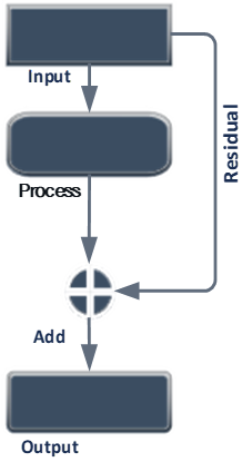
To address the degradation issue in neural networks, skip-connections are utilized, allowing specific layers in the architecture to be bypassed, as shown in Figure 2, enabling the previous layer's output to be directly fed into the current position. When the network weights approach zero, the output also approaches zero, which can cause the problem of vanishing values in the network. However, adding a skip connection, which applies an identity function, can increase the training speed. Additionally, using a 1×1×1 convolution can help control the dimension of the output. In deep learning, a residual layer refers to a neural network layer used in residual networks. The residual layer is designed to solve the issue of vanishing gradients, which can occur in deep neural networks when using certain activation functions like sigmoid or hyperbolic tangent [20, 21]. The equation for a residual layer that written as follows:
$y=f(x+r)$
where, x refers to the input to the layer, passed through a series of operations, such as convolution or pooling. The r is a skip-connections that bypasses these operations and adds the original input directly to the y output of the layer. The + operator in the equation represents the element-wise addition of the input and the residual connection.
Consider a residual block consisting of stacked layers that add values, while some layers simply output zero. However, through the use of residual blocks, the network is able to retain the weights and continually improve accuracy. In fact, it is easier to drive the residual, F(x), towards zero than to fit an identity mapping using a series of non-linear layers. Skip connections are a valuable tool in overcoming the degradation problem that arises in deeper neural networks [20].
Figure 1. Stander U-Net [19]
Figure 2. Residual block
The proposed research introduces an internal skip connection layer into the Inner Residual U-Net architecture, leveraging the well-known properties of skip connections in addressing challenges related to vanishing gradients and improving training efficiency in deep neural networks. This architectural enhancement is aligned with the research goal of enhancing the model's performance, reducing its complexity, and optimizing computational operations.
To implement the proposed approach, skip connection layers are incorporated within each block of both the encoding and decoding paths. Figure 3 illustrates the central architecture of the Residual U-Net, highlighting the strategic placement of these skip connections. By introducing this integration, the network becomes adept at capturing and propagating essential information across different scales, thereby significantly improving its ability to accurately identify affected brain regions.
Figure 3. Residual U-Net main architecture
The training of the proposed network is conducted using a curated brain images and masks. Satisfactory results have been achieved through the application of the Residual Block with U-Net, a technique that will be comprehensively discussed in subsequent sections of this paper. Importantly, it should be noted that during the training phase, the use of BraTS 2020 multimodal scans may lead to varying sizes in the input data.
The incorporation of skip connections and the utilization of multimodal scans in our Inner Residual U-Net architecture aim to advance the automatic identification of affected brain regions. This research contribution is expected to significantly enhance both the accuracy and efficiency of brain region detection, with potential implications for applications such as partial image encryption.
5.1 Pre-processing
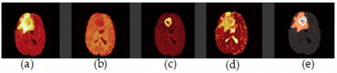
The BRATS2020 dataset comprises medical images of brain tumors in four types, namely T1, T2, FLAIR, and T1CE, as shown in Figure 4. Before processing these images, specific pre-processing steps had to be undertaken. The images were in NII format; each file contained all four types, with 155 slices for each type. However, a problem was encountered with one name of one file, and it was necessary to rename it to enable sequential data reading. Apart from the images, masks were also present that contained four values representing different types of brain cells, with values of 0, 1, 2, and 3 (where four were replaced by 3 for sequential ordering and reduced values were used). T1CE was deemed superior to T1, so it was chosen as a replacement. Subsequently, the T1CE, T2, and FLAIR images were merged into a single npy file. To optimize network training, redundant pixels with zero values were removed from the beginning and end of the merged file, specifically pixels before 56 and after 184. This step was necessary due to a black pixel frame surrounding the images.
Figure 4. Brain tumour MRI modalities. (a) FLAIR, (b): T1-weighted, (c): T1ce respectively, (d): T2-weighted and (e): Ground truth
Additionally, since the images were captured in 3D, any space at the beginning and end of the capture that did not contain helpful brain data was removed. As a result, the final merged file had a reduced size, specifically 128×128×128. This pre-processing procedure, including removing redundant zero-value pixels and empty space, ensures that the subsequent analysis and training of the Inner Residual U-Net model are performed on an optimized dataset with a consistent and appropriate image size.
5.2 The residual U-Net
The network comprises of two primary components: an encoding and a decoding layers, as shown in Figure 5. The first and last parts contain blocks that rely on the number of filters used to train the neural network. The final part is a loop connecting the two other parts. In the encoding process, each block comprises a stack of layers that take input from the preceding block and give output to the following block. There is also a linkage between each encoder block and decoder block that corresponds to it, as shown in Figure 5.
Figure 5. Outline of proposed inner residual U-Net
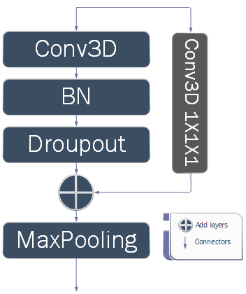
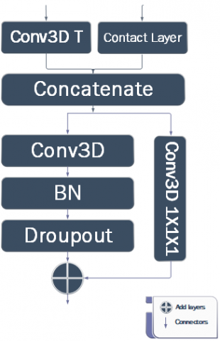
Each set comprises several successive layers, including convolution, batch normalization, dropout, add layer, and max pooling. To explain further, the encoding process involves multiple blocks, where each block applies a set of operations to the input and passes the output to the next block. The filters are learned through training the neural network, and their number determines the complexity of the layer. After the input passes through all layers, the final output is fed into the bridge, which transfers the encoded data to the decoding part of the network. The decoding process is the reverse of the encoding process, with the input being the encoded data received from the bridge. Each layer applies inverse filters to the input and passes the output to the next layer until the final decoded output is obtained. Several successive operations are performed in each set of layers, including convolution, batch normalization, dropout, add layer, and max pooling. The convolution operation applies a linear function to the output of each layer to introduce linearity into the network. Batch normalization is used to normalize the output of each layer, making it easier for the subsequent layer to process. Dropout is a technique used to mitigate the vanishing gradient problem, where the gradient values become very small during back propagation, hindering the training process. Layer addition is used to combine the outputs of two or more layers, and maximum pooling is used to down sample the output of a layer to reduce its size.
Figure 6. Encoder block
Figure 7. Decoder block
5.2.1 Encoding
The network is divided into several blocks in the encoding stage, which can be increased or decreased depending on the image size and filters used. These divisions directly affect the results of the neural network and the number of parameters used. Our approach involves adding a skip connection to each block, as illustrated in Figure 6. We take a copy of the input and pass it through a 1×1×1 convolutional layer, which is then merged with the output to preserve the block's results from vanishing gradients. We have also removed one of the convolutions from the layers in each block to reduce computation and training time. The entire network operates on 21 convolutional layers, less than what was used in the original paper [19] that used the standard U-Net without any additions. This makes learning the network more efficient, but as we know, learning requires time or high-spec GPU devices. Figure 6 shows that the encoding block contains several layers. First, the input is split into two copies. The first copy enters the 3×3×3 convolutional layers sequentially. Batch normalization is then applied, allowing us to use much higher learning rates, which increases the speed of network training. Afterwards, hierarchical down sampling is performed, and the output of both copies is concatenated. The second copy of the input undergoes a 1×1×1 convolution to assign each pixel from the input to its corresponding output pixel in all channels. The outputs of the first and second copies are then concatenated after all the operations performed on them. To achieve the U-shape of the network, the output size is reduced using MaxPooling3D 2×2×2 after the end of each.
5.2.2 Decoding
Based on the Figure 7, it illustrates the decoding process that differs from the encoding part. The input consists of two parts: one from the previous block and the other from the corresponding block in the encoding section. The first part enters the convolutional transpose, doubling the input size to match the second input from the encoding section. These two inputs are then added. The following steps are performed sequentially on the result of the previous addition. The output of the previous operation is duplicated and goes through similar processes as the encoding section, including convolutional, batch normalization, and dropout. Finally, this is merged with the second copy that has already entered the 1×1×1 convolutional layers. Table 1 shows the Network Structure of residuals and the number of required parameters.
Table 1. Network structure of residual
|
|
Unit Level |
Conv Layer |
Filter Size |
No. of Parameters |
|
Input |
|
|
0 |
|
|
Encoding |
Level 1 |
Res block MaxPooling3D |
3×3×3 / 16 2×2×2 |
6928 0 |
|
Level 2 |
Res block MaxPooling3D |
3×3×3 / 32 2×2×2 |
27,680 0 |
|
|
Level 3 |
Res block MaxPooling3D |
3×3×3 / 64 2×2×2 |
110,656 0 |
|
|
Level 4 |
Res block MaxPooling3D |
3×3×3 /128 2×2×2 |
442,496 0 |
|
|
Bridge |
Res block |
3×3×3 / 256 |
1,769,728 |
|
|
Decoding |
Level 5 |
concatenate Res block |
2×2×2 3×3×3 /128 |
0 884,864 |
|
Level 6 |
concatenate Res block |
2×2×2 3×3×3 / 64 |
0 221,248 |
|
|
Level 7 |
concatenate Res block |
2×2×2 3×3×3 / 32 |
0 55,328 |
|
|
Level 8 |
concatenate Res block |
2×2×2 3×3×3 / 16 |
0 13,840 |
|
|
Output |
|
Conv |
1×1×1 |
68 |
6.1 Experiment setup
Implemented using both Google Colab Professional. and the following pre-existing programming libraries were utilized: Keras, Glob, Scikit-Image, and others. The proposed system was applied to the Brats 2020 database. After image pre-processing and cropping the critical part of the image, a database of 128×128×128 (number of slices, length, and width) was created. The images were divided into 20% for validation and 80% for training. The model was trained using the NADAM optimizer and the learning rate is 0.0001, dice loss and focal loss functions. The dropout rate gradually increased in proportion to the network level. Image inference using the model takes between 40-80 milliseconds.
6.2 Evaluation metrics
A Python script will be written to implement the pre-processing steps. The script will take the input MRI images, apply the pre-processing steps, and save the pre-processed images in a new folder. The pre-processed images will also be visually inspected to ensure the pre-processing steps are correctly applied. NumPy will use the following libraries for numerical computing and Nibabel: for working with NII files.
The importance of pre-processing medical images before using them for diagnosis and analysis has been demonstrated. A dataset of MRI brain images has been used, and various pre-processing steps have been applied to enhance the quality of the images. The Python script is a simple but effective way to pre-process medical images and can be adapted to different medical images and pre-processing steps.
Evaluation metrics are crucial in assessing the performance of brain tumor segmentation algorithms or systems. These metrics provide quantitative measures to evaluate how well the system can delineate and segment tumor regions in medical images, like MRI scans. Here are a few commonly used evaluation metrics in brain tumor segmentation.
Primarily use the IoU (Intersection over Union) metric in our research as it measures the degree of similarity between the predicted images by the model and the ground truth images. The resulting metric is between 0 and 1, where a value closer to 1 indicates good performance, and a value less than 0.5 indicates poor performance. As shown in Eq. (1). IoU=(Intersection of predicted and ground truth)/(Union of predicted and ground truth).also there is deferent in accuracy illustrated in Eq. (2). The (DSC) Dice coefficient score is a validation metric that measures the spatial overlap between two sets of data. Precision is calculated as the positive predictive value of accurately categorized positive samples out of the numbers of all samples labelled as positive. It assesses a model's accuracy in identifying positive samples. Sensitivity is a metric used to evaluate A model's ability to predict true positives and true negatives for each category is measured by sensitivity and specificity respectively [22, 23].
Accuracy $=\frac{T P+T N}{T P+T N+F P+F N}$ (1)
$I O U=\frac{\text { Area of OverLap }}{\text { Area of Union }}$ or $I O U=\frac{T P}{T P+F P+F N}$ (2)
$D S C=\frac{2 * T P}{2 * T P+F P+F N}$ (3)
Precision $=\frac{T P}{T P+F P}$ (4)
Specificity $=\frac{T N}{T N+F P}$ (5)
Sensitivity $=\frac{T P}{T P+F N}$ (6)
where, the term TP "True Positives" refers to the count of pixels accurately identified as belonging to the object being detected. Conversely, FP "False Positives" refers to the count of pixels incorrectly classified as part of the object. FN "False Negatives" represents the number of pixels that should have been identified as part of the object but were not. TN "True Negatives" are the pixels correctly identified as not belonging to the detected object.
These metrics are widely used in brain tumor segmentation studies and effectively evaluate the performance of various algorithms and techniques. However, it's important to choose of evaluation metrics may vary depending on the specific requirements and characteristics of the proposed system [23, 24].
6.3 Result and discussion
The proposed system was evaluated on the Brats 2020 database, the result of these system as shown in Figure 8, and the Evaluation was conducted using different evaluation metrics, including sensitivity, specificity, accuracy, and Dice coefficient score.
As is evident from the results in Table 2, the proposed method yielded the best results with the least number of parameters. These results were expected due to the advantages of Skip connections, previously mentioned in reducing overfitting and addressing vanishing problems. The number of parameters in the proposed method was less than 3 million, on average, a reduction of approximately 50%. This parameter reduction led to decreased computational complexity, saving time and space during the training and testing phases.
Table 2. U-Net vs proposed res. metrics
|
|
Trainable Params |
Mean IoU |
Accuracy |
|
U-Net |
5,645,828 |
0.834 |
0.988 |
|
Proposed U-Net |
2,767,620 |
0.910 |
0.992 |
Figure 8. Examples of brain tumor segmentation
Table 3. Comparison of related works and the proposed method
|
Method |
Zhang et al. [12] |
Atiyah and Ali [16] |
He et al. [20] |
Zhang et al. [25] |
Müller [22] |
Bakas et al. [23] |
Proposed Residual UNet |
|
|
UNet++ |
EA-UNet |
|||||||
|
Accuracy |
- |
- |
- |
0.93 |
- |
0.91 |
0.957 |
0.968 |
|
Mean IoU |
0.872 |
0.9379 |
0.92 |
0.73 |
0.838 |
0.89 |
0.869 |
0.91 |
|
Mean DSC |
- |
- |
- |
- |
0.911 |
- |
- |
0.999 |
|
Precision |
- |
- |
- |
- |
- |
- |
- |
0.967 |
|
Specificity |
0.985 |
0.99 |
- |
- |
- |
- |
- |
0.989 |
|
Sensitivity |
0.883 |
0.945 |
- |
- |
- |
- |
- |
0.967 |
Figure 9 shows the original images, their masks, and predication images. The system achieved a sensitivity of 0.967, specificity of 0.989, Mean IoU of 0.910, accuracy of 0.968, and Dice coefficient score of 0.999 on the test set. These results indicate that the proposed system performs accurately in segmenting brain tumors in MRI images. Furthermore, the impact of different factors on the system's performance is analyzed. It notices that increasing the number of layers in the network improved the performance while increasing the learning rate beyond a certain threshold led to overfitting. Additionally, combining the focal loss function with the dice loss function improved the system's handling of class imbalance.
Figure 9. Accuracy & IoU of original and proposed system
6.4 Comparative study
In addition, the evaluation of the proposed system performance with the methods on the Brats 2020 database as indicated in the Table 3. Our system outperformed most of the existing methods in terms of accuracy and Dice coefficient score. This demonstrates the effectiveness of the proposed system in brain tumor segmentation.
The proposed system implements a U-Net architecture with four encoding layers, a bridge layer, and a loss function (Focal loss and Dice loss). It was noticed that the proposed trained model for 100 epochs obtained a Mean IoU of 0.910 and an accuracy of 0.968.
The Enhancing residual blocks make the network realize the residual mapping between input and output as a substitute for a direct mapping between them, so that model can rapidly learn residual mapping corresponding to block residual technology.
In conclusion, implementing a deep learning model for segmentation of medical image on the BRATS2020 dataset seems to have achieved a good performance, as indicated by high IoU and accuracy values. However, it is essential to understand that there is not a universal solution for this issue, and the good approach that depend on the distinct attributes of the dataset and the situation at hand that aim to solve. It is essential to try different techniques and approaches and carefully evaluate their impact on the model's performance. The proposed system achieved promising results in segmenting brain tumors in MRI images and outperformed most existing methods on the Brats databases, as mentioned in section 6.4. The results suggest that the proposed system used for brain tumor segmentation in clinical practice.
The objective in the future is to assess the performance of the proposed enhanced Residual U-Net architecture on other medical imaging datasets beyond the BraTS2020 dataset to evaluate its generalizability, and this would involve exploring how the architecture performs on diverse datasets that cover a range of medical conditions and imaging modalities. For instance, datasets related to lung imaging, retinal scans, or cardiac imaging could offer unique perspectives on the effectiveness of the proposed architecture in different medical domains; by analyzing the architecture's performance on various datasets, and can get a comprehensive understanding of its strengths and limitations in different contexts.
Exploring the impact of hyperparameter tuning on the performance of the proposed enhanced Residual U-Net architecture, such as varying the number of encoding and decoding layers, the learning rate, or filters numbers in the convolutional layers.
The impact of different loss functions on the performance of the proposed enhanced Residual U-Net architecture was assessed. While Focal loss + Dice loss has illustrated good results in medical image segmentation, it is essential to compare its performance with other commonly employed loss functions such as binary cross-entropy or weighted cross-entropy. This comparison analysis will offer insights into the cons and bons of different loss functions and their suitability for specific segmentation tasks and medical imaging datasets. We can refine the architecture's training process by considering alternative loss functions and potentially accomplishing more accurate and reliable segmentation results.
[1] Tiwari, A., Srivastava, S., Pant, M. (2020). Brain tumor segmentation and classification from magnetic resonance images: Review of selected methods from 2014 to 2019. Pattern Recognition Letters, 131: 244-260. https://doi.org/10.1016/j.patrec.2019.11.020
[2] Addeh, A., Iri, M. (2021). Brain tumor type classification using deep features of MRI images and optimized RBFNN. ENG Transactions, 2: 1-7.
[3] Muhammad, K., Khan, S., Del Ser, J., De Albuquerque, V.H.C. (2020). Deep learning for multigrade brain tumor classification in smart healthcare systems: A prospective survey. IEEE Transactions on Neural Networks and Learning Systems, 32(2): 507-522. https://doi.org/10.1109/TNNLS.2020.2995800
[4] Cui, S., Mao, L., Jiang, J., Liu, C., Xiong, S. (2018). Automatic semantic segmentation of brain gliomas from MRI images using a deep cascaded neural network. Journal of Healthcare Engineering, 2018: 4940593. https://doi.org/10.1155/2018/4940593
[5] Zhou, C., Chen, S., Ding, C., Tao, D. (2019). Learning contextual and attentive information for brain tumor segmentation. In Brainlesion: Glioma, Multiple Sclerosis, Stroke and Traumatic Brain Injuries: 4th International Workshop, BrainLes 2018, Granada, Spain, pp. 497-507. https://doi.org/10.1007/978-3-030-11726-9_44
[6] Moeskops, P., Viergever, M.A., Benders, M.J., Išgum, I. (2015). Evaluation of an automatic brain segmentation method developed for neonates on adult MR brain images. In Medical Imaging 2015: Image Processing, 9413: 304-309. https://doi.org/10.1117/12.2081833
[7] Mendrik, A.M., Vincken, K.L., Kuijf, H.J., Breeuwer, M., Bouvy, W.H., De Bresser, J., Viergever, M.A. (2015). MRBrainS challenge: Online evaluation framework for brain image segmentation in 3T MRI scans. Computational Intelligence and Neuroscience, 2015: 1-16. https://doi.org/10.1155/2015/813696
[8] Balafar, M.A., Ramli, A.R., Saripan, M.I., Mashohor, S. (2010). Review of brain MRI image segmentation methods. Artificial Intelligence Review, 33: 261-274. https://doi.org/10.1007/s10462-010-9155-0
[9] Despotović, I., Goossens, B., Philips, W. (2015). MRI segmentation of the human brain: challenges, methods, and applications. Computational and Mathematical Methods in Medicine, 2015: 450341. https://doi.org/10.1155/2015/450341
[10] Thillaikkarasi, R., Saravanan, S. (2019). An enhancement of deep learning algorithm for brain tumor segmentation using kernel based CNN with M-SVM. Journal of Medical Systems, 43: 1-7. https://doi.org/10.1007/s10916-019-1223-7
[11] Ciresan, D., Giusti, A., Gambardella, L., Schmidhuber, J. (2012). Deep neural networks segment neuronal membranes in electron microscopy images. Advances in Neural Information Processing Systems, 25.
[12] Zhang, Z., Liu, Q., Wang, Y. (2018). Road extraction by deep residual U-Net. IEEE Geoscience and Remote Sensing Letters, 15(5): 749-753. https://doi.org/10.1109/LGRS.2018.2802944
[13] Salman, L.A., Hashim, A.T., Hasan, A.M. (2022). Selective medical image encryption using polynomial based secret image sharing and chaotic map. International Journal of Safety and Security Engineering, 12(3): 357-369. https://doi.org/10.18280/ijsse.120310
[14] Aghalari, M., Aghagolzadeh, A., Ezoji, M. (2021). Brain tumor image segmentation via asymmetric/symmetric UNet based on two-pathway-residual blocks. Biomedical Signal Processing and Control, 69: 102841. https://doi.org/10.1016/j.bspc.2021.102841
[15] Xiao, Z., Du, M., Liu, J., Sun, E., Zhang, J., Gong, X., Chen, Z. (2023). EA-UNet based segmentation method for OCT image of uterine cavity. In Photonics, 10(1): 73. https://doi.org/10.3390/photonics10010073
[16] Atiyah, A.Z., Ali, K.H. (2021). Brain MRI images segmentation based on U-Net architecture. IJEEE Journal, 18: 21-27. https://doi.org/10.37917/ijeee.18.1.3
[17] Walsh, J., Othmani, A., Jain, M., Dev, S. (2022). Using U-Net network for efficient brain tumor segmentation in MRI images. Healthcare Analytics, 2: 100098. https://www.sciencedirect.com/science/article/pii/S2772442522000429.
[18] Kim, P. (2017). MATLAB Deep Learning. Apress. https://doi.org/10.1007/978-1-4842-2845-6
[19] Ronneberger, O., Fischer, P., Brox, T. (2015). U-Net: Convolutional networks for biomedical image segmentation. In Medical Image Computing and Computer-Assisted Intervention–MICCAI 2015: 18th International Conference, Munich, Germany, pp. 234-241. https://doi.org/10.1007/978-3-319-24574-4_28
[20] He, K., Zhang, X., Ren, S., Sun, J. (2016). Deep residual learning for image recognition. In Proceedings of the IEEE Conference on Computer Vision and Pattern Recognition, Las Vegas, NV, USA, pp. 770-778. https://doi.org/10.1109/CVPR.2016.90
[21] Chen, X., Yao, L., Zhang, Y. (2020). Residual attention u-net for automated multi-class segmentation of covid-19 chest CT images. arXiv preprint arXiv:2004.05645. https://arxiv.org/abs/2004.05645
[22] Müller, D., Soto-Rey, I., Kramer, F. (2022). Towards a guideline for evaluation metrics in medical image segmentation. BMC Research Notes, 15(1): 1-8. https://doi.org/10.1186/s13104-022-06096-y
[23] Bakas, S., Akbari, H., Sotiras, A., Bilello, M., Rozycki, M., Kirby, J.S., Davatzikos, C. (2017). Advancing the cancer genome atlas glioma MRI collections with expert segmentation labels and radiomic features. Scientific Data, 4(1): 1-13. https://doi.org/10.1038/sdata.2017.117
[24] Havaei, M., Davy, A., Warde-Farley, D., Biard, A., Courville, A., Bengio, Y., Larochelle, H. (2017). Brain tumor segmentation with deep neural networks. Medical Image Analysis, 35: 18-31. https://doi.org/10.1016/j.media.2016.05.004
[25] Zhang, Y., Mehta, S., Caspi, A. (2021). Rethinking semantic segmentation evaluation for explain ability and model selection. arXiv preprint arXiv:2101.08418. https://doi.org/10.48550/arXiv.2101.08418