Wala’a A. Mahdi*![]() | Sadiq Al-Nassir
| Sadiq Al-Nassir![]()
© 2024 The authors. This article is published by IIETA and is licensed under the CC BY 4.0 license (http://creativecommons.org/licenses/by/4.0/).
OPEN ACCESS
This study examines a fractional-order prey-predator model incorporating fear effects and harvesting impacts on prey dynamics, employing both continuous and discretized frameworks with the Monod–Haldane functional response. The existence, uniqueness, and boundedness of the system's solutions, along with their non-negativity, are established through rigorous analysis. The system is further evaluated for potential equilibrium points, with their stability conditions meticulously assessed. It is revealed that the model possesses three locally stable equilibrium points, provided certain conditions are met. In the context of the discretized model, an optimal harvesting strategy is formulated, guided by Pontryagin’s Maximum Principle, to ensure maximum economic yield. Numerical simulations complement the analytical findings, offering insights into the system's dynamic behavior under both continuous and discrete scenarios. Moreover, the optimality problem associated with harvesting strategies is resolved. The study concludes by summarizing the significant outcomes and their implications for ecological management.
fear effect, Monod–Haldane functional response, harvesting, Caputo fractional derivative, Pontryagin’s maximal principle
Predation is a key ecological interaction that affects populations and communities. This interaction can directly modify by the kinetic effects of relationship on biological rates and indirectly through integrated behavioral and morphological responses of the populations including the study of forms mutations, adaptation and evolution, the consideration of the features and structure of organisms and their place in the greater environment [1]. The fear effect is one of many aspects that controls the dynamic behaviors of prey-predator systems due to its impact on the population abundant of the prey [2]. Zhang et al. [3], Cresswell [4], Xu [5] showed that the fear that consider by the predator is greater effect on the prey species than the direct killing. Lan et al. [6] interpreted that the fear effect may occur from not only adult predators but also from juvenile one. Fractional derivatives and integrals have provided a better tool to understanding some biological models, especially differential equations models have been interested due to the memory effect which exists in most biological systems [7, 8].
The concept of the optimal harvesting has an important significant effect in treating the renewable stocks due the economic feature and to maintain and prevent the species away from the extinction, so that many authors and researchers are widely considered and discussed this subject in their papers [9-14].
The Caputo fractional order derivatives are considered because the fractional order initial conditions are not necessary to define and the fractional-order derivative of constant function is equal to zero [15, 16].
Difference equations are well used to describe the dynamic process the life of many populations that cannot be encompassed by other simple continuous equations for example, plants, in the pacific salmon fishery, bird and mammals, population of insects, and others. In spite of their apparent simplicity discrete time models are frequently used and employed, these models can show and exhibit amazingly complex dynamic behavior [17-21].
In this article, we consider and investigate a non-integer order derivative prey-predator biological model with its discretization.
Functional response can greatly affect model predations, thus some functional responses are employed and considered to depict and describe this phenomenon. For example, the Holling functional response of type I, II and III, as well as, Beddingto-De Agelis and Crowley-Martin functional response are widely used in the literatures [1, 22, 23]. Another type of functional response which is known as Monod–Haldane function that has the form $\psi(N)=\frac{r N}{a+b N+N^2}$, where r, a and b are positive constants which is introduced and considered by Dai et al. [24], while Andrews [25] presented a simple form of the Monod–Haldane functional response.
The Monod–Haldane functional response is also used in the system. In addition, the effect of fear on prey species and harvesting are studied.
The structure of this work is as follows: In section 2, the mathematical fractional-order model is formulated so, the mathematical results and behaviors dynamics for the suggested model are discussed. The existence and uniqueness as well as the boundedness and non-negativity of the solutions are shown. We also investigate the local stability of all equilibrium points of the considered system. In section 3, the discretization process is done and the local stability of its l equilibria are studied and investigated. The Pontryagin’s maximum principle is used and applied to obtain the optimal harvest amount for the discrete model in section 4. Numerical outcomes are given and presented in section 5 to get the optimality problem and to confirm the mathematical analysis. In section 6, the conclusion of the results of this work is given.
Wang et al. [2] studied and discussed the fear effect in prey-predator model with the Holling’s type II functional response. Their model is giving as follows:
$\left.\begin{array}{c}\frac{d n(t)}{d t}=\frac{r_0 n(t)}{1+k p(t)}-d n(t)-c n^2(t)-\frac{n(t) p(t)}{1+b n(t)} \\ \frac{d p(t)}{d t}=\frac{e n(t) p(t)}{1+b n(t)}-f p(t)\end{array}\right]$ (1)
where, n(t) and p(t) are the size of prey and predator species at time t, respectively. The interpretation of the parameters r0, k, d, c, e and f are given in Table 1.
Table 1. Parameters' description
|
Parameter |
Description |
Parameter |
Description |
|
r0 |
The rate of birth in the prey species. |
e |
The conversion rate of prey’s size to predator’s size. |
|
d |
The natural death rate of the prey. |
f |
The rate of death in the predator species. |
|
c |
The death rate due to intraspecies competition. |
k |
The level of fear in the prey. |
Now, we introduce a fractional-q-order derivatives by using the Caputo’s definition where $q \in(0,1)$ [13], with a simplest form of Monod–Haldane function [24]. We also consider that the prey is exposed to a constant rate harvesting then in later section we consider the non-harvesting rate. Therefore, the model (1) becomes as follows:
Therefore, the model (1) becomes as follows:
$\left.\begin{array}{c}\mathcal{D}^q n(t)=\frac{r_0 n(t)}{1+k p(t)}-d n(t)-c n(t)^2-\frac{r n(t) p(t)}{a+n(t)^2}-h n(t) \\ \mathcal{D}^q p(t)=\frac{\operatorname{ern}(t) p(t)}{a+n(t)^2}-f p(t)\end{array}\right]$ (2)
where, r is the capture rate of the predator and a is the reciprocal of group defense in prey. Some properties to the fractional-order derivatives can be found in reference [13, 23, 26] that are needed throughout this paper. Next theorems give the existence, uniqueness for the system (2).
Theorem (1): Let η be a sufficiently large, the considered system (2) has a unique solution (n(t), p(t)) in F×(0, T] at any non-negative initial value (n0, p0), for all t>0, where $F=\left\{(n, p) \in R^2:(|n|,|p|) \leq \eta\right\}$.
Proof: We first assume that $X=(n, p), \hat{X}=(\hat{n}, \hat{p})$, and then consider a mapping B(X)=(B1(X), B2(X)), such that $B_1(X)=\frac{r_0 n}{1+k p}-d n-c n^2-\frac{r n p}{a+n^2}-h n, B_2(X)=\frac{e r n p}{a+n^2}-f p$. For X, $\hat{X} \in F$ and by simple computations, one can easily get the following:
$\begin{gathered}\|B(X)-B(\hat{X})\|=\left|B_1(X)-B_1(\hat{X})\right|+\left|B_2(X)-B_2(\hat{X})\right| \leq r_0|n(1+k \hat{p})-\hat{n}(1+k p)|+c|(n-\hat{n})(n+\hat{n})|+ \\ d|n-\hat{n}|+h|n-\hat{n}|+r\left|n p\left(a+\hat{n}^2\right)-\hat{n} \hat{p}\left(a+n^2\right)\right|+ \\ \operatorname{er}\left|n p\left(a+\hat{n}^2\right)-\hat{n}\left(a+n^2\right)\right|+f|p-\hat{p}| \leq L\|X-\hat{X}\|\end{gathered}$
where, $L=\max \left\{\left(r_0+r_0 k \eta+d+2 c \eta+h+r \eta a(1+e)+r \eta^2(1+e),\left(r \eta a(1+e)+r \eta^2(1+e)+r_0 k \eta+f\right)\right\}\right.$. Hence, B(X) has the Lipschitz condition. Therefore, there exists a unique solution to the fractional order system (2).
The non-negativity and boundedness of solutions of system (2) are proved by the following theorem.
Theorem (2): For the system (2) with n0 and p0, all solutions that start in F+ are uniformly bounded and non-negative, where F+={n≥0, p≥0}.
Proof: Consider a function $V=n+\frac{p}{e}$ and the initial values are n0 and p0 so that $D^q V(t)+\mu V(t)=D^q n(t)+\frac{1}{e} D^q p(t)+\mu V(t)$. Then DqV(t)+μV(t)≤K when μ<f. where, $K=\frac{\left(r_0-d-h+\mu\right)^2}{4 c^2}$.
Therefore, by using the comparison theorem that presented in reference [14], we have $V(t) \leq\left(V(0)-\frac{K}{\mu}\right) E_q\left[-\mu t^q\right]+K$, and
$0 \leq V(t) \leq K$ ast $\rightarrow \infty$ (3)
Hence, all solutions to system (2) are uniformly bounded.
In order to prove the non-negativity solution, we first notice that from the first equation of system (2).
$D^q n(t)=\frac{r_0 n}{1+k p}-d n-c n^2-\frac{r n p}{a+n^2}-h n$
And from Eq. (3), we have $n+\frac{p}{e} \leq \frac{\left(r_0-d-h+\mu\right)^2}{4 c^2 \mu}=\mu_1$. Then, we get: $\begin{aligned} & D^q n(t)=\frac{r_0 n}{1+k p}-d n-c n^2-\frac{r n p}{a+n^2}-h n \geq-(d+h+ \left.c \mu_1\right) n=\varphi_1 n\end{aligned}$.
This implies: $n(t) \geq n_0 E_q\left(\varphi_1 t^q\right)$. where, φ1=-(d+h+cμ1).
Since Eq(t)>0, for any order q in (0, 1), then as n(t)≥0, for all t>0.
From the second equation in Eq. (2), it is clear that Dqp(t)≥-fp. So that, p(t)≥p0Eq(-ftq)≥0 for all t>0.
Hence, the fractional order system (2) has non-negative solutions.
To find all possible equilibria of the system (2), the following equations have to be solved:
$\left.\begin{array}{c}\mathcal{D}^q n(t)=\frac{r_0 n(t)}{1+k p(t)}-d n(t)-c n(t)^2-\frac{r n(t) p(t)}{a+n(t)^2}-h n(t)=0 \\ \mathcal{D}^q p(t)=\frac{\operatorname{ern}(t) p(t)}{a+n(t)^2}-f p(t)=0\end{array}\right]$ (4)
Therefore, the equilibria of the system (2) are as follows:
1. The extinction equilibrium point e0=(0, 0) always exists.
2. The free predator point equilibrium point $e_1=\left(n^*, 0\right)=\left(\frac{r_0-(d+h)}{c}, 0\right)$ exists if r0>d+h.
3. The interior or positive equilibrium point e2=(n*, p*) where n* and p* are the positive roots the following equations, respectively: $f n^{*^2}-e r n^*+a f=0$, $\begin{aligned} & k p^{*^2}+\left(r+\left(d+c n^*+h\right) k\left(a+n^{* 2}\right)\right) p^*+((d+ \left.\left.c n^*+h\right)-r_0\right)\left(a+n^{*^2}\right)=0 \end{aligned}$.
The general variation matrix of the suggested model (2) at any point (n, p) is then as follows:
$J=\left[\begin{array}{cc}\frac{r_0}{1+k p}-d-2 c n-h+\frac{r p n^2-a r p}{\left(a+n^2\right)^2} & -\frac{r_0 k n}{(1+k p)^2}-\frac{r n}{\left(a+n^2\right)} \\ \frac{e r a p-e r p n^2}{\left(a+n^2\right)^2} & \frac{e r n}{\left(a+n^2\right)}-f\end{array}\right]$
So, the characteristic polynomial of J is as follows:
P(λ)=λ2+a2λ+a1=0
where,
$\begin{gathered}a_2=-\left(\frac{r_0}{1+k p}-d-2 c n-h+\frac{r p n^2-a r p}{\left(a+n^2\right)^2}+\frac{e r n}{\left(a+n^2\right)}-f\right) \text { and } a_1=\left(\frac{r_0}{1+k p}-d-2 c n-h+\frac{r p n^2-a r p}{\left(a+n^2\right)^2}\right)\left(\frac{e r n}{\left(a+n^2\right)}-f\right)+ \left(\frac{r_0 k n}{(1+k p)^2}+\frac{r n}{\left(a+n^2\right)}\right)\left(\frac{e r a p-e r p n^2}{\left(a+n^2\right)^2}\right) .\end{gathered}$
The next Theorem establishes the local stability of the suggested system (2).
Theorem (3): The local stability of equilibria of system (2) are as follows:
1. The trivial equilibrium point e0=(0, 0) is locally stable, if d+h>r0.
2. The free predator equilibria point $e_1=\left(\frac{r_0-(d+h)}{c}, 0\right)$ is locally stable, if d+h<r0 and $\frac{\operatorname{cer}\left(r_0-(d+h)\right)}{a c^2+\left(r_0-(d+h)\right)^2}<f$.
3. The interior or positive equilibrium point, (n*, p*) is locally stable if one of the following conditions holds:
I. a2>0 and a1>0.
II. a2<0, $4 a_1>a_2^2$ and $\left|\tan ^{-1}\left(\frac{\sqrt{4 a_1-a_2^2}}{a_2}\right)\right|>q \frac{\pi}{2}$.
where,
$a_2=-\left(\frac{r_0}{1+k p^*}-d-2 c n^*-h+\frac{r p^* n^{* 2}-a r p^*}{\left(a+n^{* 2}\right)^2}+\frac{e r n^*}{\left(a+n^{* 2}\right)}-f\right) and \,\,\begin{gathered}a_1=\left(\frac{r_0}{1+k p^*}-d-2 c n^*-h+\frac{r p^* n^{* 2}-a r p^*}{\left(a+n^{* 2}\right)^2}\right)\left(\frac{e r n^*}{\left(a+n^{* 2}\right)}-f\right) +\left(\frac{r_0 k n^*}{\left(1+k p^*\right)^2}+\frac{r n^*}{\left(a+n^{* 2}\right)}\right)\left(\frac{e r a p^*-e r p^* n^{* 2}}{\left(a+n^{* 2}\right)^2}\right) .\end{gathered}$
Proof:
1. At the point e0=(0, 0), the Jacobian matrix J of the suggested system (2) is:
$J\left(e_0\right)=\left[\begin{array}{cc}r_0-(d+h) & 0 \\ 0 & -f\end{array}\right]$
Since the eigenvalues of J(e0) are λ1=r0-(d+h) and λ2=-f, then we get $\left|\arg \left(\lambda_1\right)\right|>q \frac{\pi}{2}$ if d+h>r0 and $\left|\arg \left(\lambda_2\right)\right|>q \frac{\pi}{2}$. According to the proposition 1 in reference [27], hence the point e0 is locally stable.
2. The Jacobian matrix at the point e1, J(e1) is:
$J\left(e_1\right)=\left[\begin{array}{cc}d+h-r_0 & \frac{-r_0 k\left(r_0-(d+h)\right)}{c}-\frac{c r\left(r_0-(d+h)\right)}{a c^2+\left(r_0-(d+h)\right)^2} \\ 0 & \frac{\operatorname{cer}\left(r_0-(d+h)\right)}{a c^2+\left(r_0-(d+h)\right)^2}-f\end{array}\right]$
Then, the eigenvalues of J(e1) are λ1=d+h-r0 and $\lambda_2=\frac{\operatorname{cer}\left(r_0-(d+h)\right)}{a c^2+\left(r_0-(d+h)\right)^2}-f$. Since d+h<r0, it is clear that $\left|\arg \left(\lambda_1\right)\right|>q \frac{\pi}{2} \forall q \in(0,1)$. Now if $f>\frac{\operatorname{cer}\left(r_0-(d+h)\right)}{a c^2+\left(r_0-(d+h)\right)^2}$, then $\left|\arg \left(\lambda_2\right)\right|>q \frac{\pi}{2}$. According to the study [27], the free predator point e1 is locally stable point.
3. It is easy to see that J(e2) is evaluated as:
$\begin{aligned} & J\left(e_2\right)={\left[\begin{array}{cc}\frac{r_0}{1+k p^*}-d-2 c n^*+\frac{r p^* n^{* 2}-a r p^*}{\left(a+n^{* 2}\right)^2}-h & -\left(\frac{r_0 k n^*}{\left(1+k p^*\right)^2}+\frac{r n^*}{\left(a+n^{* 2}\right)}\right) \\ \frac{e r a p^*-e r p^* n^{* 2}}{\left(a+n^{* 2}\right)^2} & \frac{e r n^*}{\left(a+n^{* 2}\right)}-f\end{array}\right]}\end{aligned}$
The characteristics polynomial of J at the point e2 is as follows: P(λ)=λ2+a2λ+a1=0.
Then according to the proposition 1 in the study [27], we get the results.
In this part, we apply the discretization process of piecewise constant arguments which is presented in references [20, 28] to the suggested fractional prey-predator dynamics system (2). These yields:
$\begin{gathered}n_{m+1}=n_m+\frac{s^q}{q \Gamma(q)}\left(\frac{r_0 n_m}{1+k p_m}-d n_m-c n_m^2\right. \left.-\frac{r n_m p_m}{a+n_m^2}-h n_m\right) \\ p_{m+1}=p_m+\frac{s^q}{q \Gamma(q)}\left(\frac{e r n_m p_m}{a+n_m^2}-f p_m\right)\end{gathered}$ (5)
where, s>0.
Now, we discuss the behaviors of the discrete fractional dynamics model (5).
We note that system (5) has the same fixed (equilibrium) points as the suggested system (2). The general variation matrix of model (5) at any fixed point (n, p) is
$J=\left[\begin{array}{cc}1+W\left(\frac{r_0}{1+k p}-d-2 c n+\frac{r p n^2-a r p}{\left(a+n^2\right)^2}-h\right) & -W\left(\frac{r_0 k n}{(1+k p)^2}+\frac{r n}{\left(a+n^2\right)}\right) \\ W\left(\frac{e r a p-e r p n^2}{\left(a+n^2\right)^2}\right) & 1+W\left(\frac{e r n}{\left(a+n^2\right)}-f\right)\end{array}\right]$.
where, $W=\frac{s^q}{q \Gamma(q)}$.
Remark:
For a discrete system a fixed point (equilibrium) is called a locally stable if all eigenvalues of its Jacobian matrix at that fixed point are inside the unit circle, otherwise it is unstable fixed point, and it is non-hyperbolic point if at least one of the eigenvalues has modules equal to 1.
Lemma (4) [17, 29]
Let $F(\xi)=\xi^2+n_1 \xi+n_2$ be the characteristic polynomial of degree two, with F(1)>0. Then the F(-1)>0 and n2<1 if and only if $\left|\xi_i\right|<1, i=1,2$.
Now, we will determine the nature of all fixed (equilibrium) points of the model (5).
Theorem (5): For the discrete model (5), the trivial equilibrium point e0is:
a. A locally stable if $r_0 \in\left(d+h-\frac{2}{W}, d+h\right)$ and $W<\frac{2}{f}$, otherwise it is unstable.
b. A non-hyperbolic point if r0=d+h or $r_0=d+h-\frac{2}{w}$ or $W=\frac{2}{f}$.
Proof: It is easy to see that J(e0) is as follows: $J\left(e_0\right)=\left[\begin{array}{cc}1+W\left(r_0-(d+h)\right) & 0 \\ 0 & 1-W f\end{array}\right]$, clearly calculations that the eigenvalues of J(e0) are λ1=1+W(r0-(d+h)) and λ2=1-Wf. Now if $W<\frac{2}{f}$, then 0<Wf<2 and |λ2|<1. Let $d+h-\frac{2}{W}<r_0<d+h$, then -2<W(r0-(d+h))<0 and |λ1|<1. Therefore, the trivial equilibrium point e0 is a locally stable. It is clear that if r0=d+h or $r_0=d+h-\frac{2}{W}$ or $=\frac{2}{f}$, then e0 is a non-hyperbolic point.
Theorem (6): The free predator fixed point $e_1=\frac{\left(r_0-(d+h)\right.}{}, 0$ of the discrete model (5) is:
a. A locally stable point if $\mathrm{W}<\frac{2}{r_0-(d+h)}$ and $f \in\left(M, \frac{2+W M}{W}\right)$, where $M=\frac{\operatorname{cre}\left(r_0-(d+h)\right)}{\left(a c^2+\left(r_0-(d+h)\right)^2\right)}$, otherwise $e_1$ is unstable point.
b. non-hyperbolic point if $\mathrm{W}=\frac{2}{r_0-(d+h)}$ or $f=M$ or $f=\frac{2+W M}{W}$.
Proof: At the free predator fixed point e1 the J(e1) is as follows:
$\begin{aligned} & J\left(e_1\right) =\left[\begin{array}{cc}1+W\left(d+h-r_0\right) & -W\left(\frac{r_0 k\left(r_0-(d+h)\right)}{c}+\frac{c r\left(r_0-(d+h)\right)}{a c^2+\left(r_0-(d+h)\right)^2}\right) \\ 0 & 1+W\left(\frac{\operatorname{cer}\left(r_0-(d+h)\right)}{a c^2+\left(r_0-(d+h)\right)^2}-f\right)\end{array}\right]\end{aligned}$
The eigenvalue s of J(e1) are λ1=1+W(d+h-r0) and $\lambda_2=1+W\left(\frac{\operatorname{cer}\left(r_0-(d+h)\right)}{a c^2+\left(r_0-(d+h)\right)^2}-f\right)$. If $W<\frac{2}{r_0-(d+h)}$, then -1<1+W(d+h-r0)<1 and |λ1|<1, while, if $M<f<\frac{2+W M}{W}$, then MW<Wf<2+WM and-1<(1+WM-Wf)<1. Hence |λ2|<1 therefore, the free predator point e1 is (a locally stable), otherwise it is unstable point. Clearly that if $\mathrm{W}=\frac{2}{r_0-(d+h)}$ or $f=M$ or $f=\frac{2+W M}{W}$ then e1 is a non-hyperbolic point. Now, we discuss the properties of stability analysis for the positive or interior point e2=(n*, p*) of system (5) and then we set the following theorem:
Theorem (7): The positive or interior point e2=(n*, p*) of a discrete system (5) is a locally stable if $f \in\left(S_3, \min \left\{S_1, S_2\right\}\right)$, where
$\begin{gathered}S_1=\frac{1-W_1-W_4+W_1 W_4-W_2 W_3}{W\left(W_1-1\right)}, \\ S_2=\frac{1+W_4+W_1+W_1 W_4-W_2 W_3}{W\left(W_1+1\right)}, \\ S_3=\frac{W_1 W_4-W_2 W_3-1}{W W_1}, \\ W_1=1+W\left(\frac{r_0}{1+k p^*}-d-2 c n^*+\frac{r p^* n^{* 2}-a r p^*}{\left(a+n^{* 2}\right)^2}-h\right), \\ W_2=-W\left(\frac{r_0 k n^*}{\left(1+k p^*\right)^2}+\frac{r n^*}{\left(a+n^{* 2}\right)}\right),W_3=W\left(\frac{e r a p^*-e r p^* n^{* 2}}{\left(a+n^{* 2}\right)^2}\right) \text { and } W_4=1+W\left(\frac{e r n^*}{\left(a+n^{* 2}\right)}\right) .\end{gathered}$
Proof: The J(e2) of the discrete system (5) is as follows: $J\left(e_2\right)=\left[\begin{array}{cc}W_1 & W_2 \\ W_3 & W_4-W f\end{array}\right]$. So, the corresponding characteristic polynomial is:
$\begin{gathered}F(\lambda)=\left(W_1-\lambda\right)\left(W_4-W f-\lambda\right)-\left(W_2 W_3\right)=0 \Rightarrow \\ W_1 W_4-W_1 W f-W_1 \lambda-W_4+W f \lambda+\lambda^2-W_2 W_3=0 \Rightarrow \\ \lambda^2-\left(W_1+W_4-W f\right) \lambda+W_1 W_4-W_1 W f-W_2 W_3=0 .\end{gathered}$
Lead to F(λ)=λ2+ppλ+qq=0. Where pp=Wf-W1-W4, and qq=W1W4-W1Wf-W2W3. Let f<S1, then fW(W1-1)<1-W1-W4+ W1W4- W2W3 and 1-W1-W4+W1W4-fWW1+fW- W2W3>0.This gives that F(1)>0. Now, if f<S2 then fW(W1+1)<1+W4+W1+W1W4- W2W3 and 1+W4+W1+W1W4-fWW1-fW-W2W3>0 this implies that F(-1)>0. Now, if f>S3, then fW1W>W1W4- W2W3-1 and W1W4-fW1W-W2W3<1 then gives that qq<1. Hence, according to Lemma (4), the interior fixed point e2 is a locally stable.
The key idea in this section is to determine how one can maximize the profits net from harvesting the prey population [30]. We follow the profits net is given as follows:
$J\left(h_t\right)=\max \sum_{t=0}^{T-1}\left(c_1 h_t n_t-c_2 h_t{ }^2\right)$ (6)
where, c1 represents the price of the harvesting, c2 is positive constant, ht is the control variable such that 0≤ht≤hmax<1, hmax which is the maximum harvest amount, T is the time horizon and $c_2 h_t^2$ is the total cost. The goal is to maximize (6) subject to the following state equations:
$\left.\begin{array}{c}n_{t+1}=n_t+\frac{s^q}{q \Gamma(q)}\left(\frac{r_0 n_t}{1+k p_t}-d n_t-c n_t^2-\frac{r n_t p_t}{a+n_t^2}-h_t n_t\right) \\ p_{t+1}=p_t+\frac{s^q}{q \Gamma(q)}\left(\frac{e r n_t p_t}{a+n_t^2}-f p_t\right)\end{array}\right]$ (7)
The Hamiltonian function is given by references [23, 28]:
$\begin{gathered}H_t=c_1 h_t n_t-c_2 h_t^2+\mu_{1, t+1}\left(n_t+\frac{s^q}{q \Gamma(q)}\left(\frac{r_0 n_t}{1+k p_t}-d n_t-\right.\right. \left.\left.c n_t^2-\frac{r n_t p_t}{a+n_t^2}-h_t n_t\right)\right)+\mu_{2, t+1}\left(p_t+\frac{s^q}{q \Gamma(q)}\left(\frac{e r n_t p_t}{a+n_t^2}-f p_t\right)\right)\end{gathered}$ (8)
where, μ1,t+1 and μ2,t+1 are the adjoint variables [28, 31]. To show the previous discrete optimal control problem, we apply the Pontryagin’s maximum principle [32]. Then, we get:
$\begin{array}{r}\mu_{1, t}=\frac{\partial H_t}{\partial n_t}=c_1 h_t+\mu_{1, t+1}\left(1+\frac{s^q}{q \Gamma(q)}\left(\frac{r_0}{1+k p_t}-d-\right.\right. 2 c n_t-h_t+\left.\left.\frac{r p_t n_t^2-a r p_t}{\left(a+n_t^2\right)^2}\right)\right)+\mu_{2, t+1}\left(\frac{s^q}{q \Gamma(q)}\left(\frac{\operatorname{erap}_t-e r p_t n_t^2}{\left(a+n_t^2\right)^2}\right)\right), \\ \mu_{2, t}=\frac{\partial H_t}{\partial p_t}=-\mu_{1, t+1}\left(\frac{s^q}{q \Gamma(q)}\left(\frac{r_0 k n_t}{\left(1+k p_t\right)^2}+\frac{\left.r+n_t^2\right)}{(a+1}\right)\right.+\mu_{2, t+1}\left(1+\frac{s^q}{q \Gamma(q)}\left[\frac{e r n_t}{\left(a+n_t^2\right)}-f\right]\right) .\end{array}$
According to the Pontryagin maximum principle, the characteristic control harvesting solution is given by the following:
$h_t^*=\left\{\begin{array}{cc}0, & \frac{\left(c_1-\mu_{1, t+1} \frac{s^q}{q \Gamma(q)}\right)}{2 c_2} n_t<0 \\ \frac{\left(c_1-\mu_{1, t+1} \frac{s^q}{q \Gamma(q)}\right)}{2 c_2} n_t, & \left.0<\frac{\left(c_1-\mu_{1, t+1} s^q\right.}{2 c_2}\right) \\ h_{\text {max }}, & h_{\max }<\frac{\left(c_1-\mu_{1, t+1} \frac{s^q}{q \Gamma(q)}\right)}{2 c_2} n_t\end{array}\right.$
In this part, we discuss and give a numerical study to enhance the above theoretical results and to confirm the dynamics behaviors of fractional prey-predator model as well as its discretization. We consider the examples to account the local stability of equilibria:
Example 1: A set of different values of parameters in Table 2 are used to illustrate and show the local stability of equilibrium points e0, e1 and e2 of the fractional predator-prey model (2). These are done according to Theorem 3.
Table 2. The values of parameters for the fixed point e0, e1 and e2for the fractional model (2)
|
Parameter’s Value |
e0 |
e1 |
e2 |
|
r0 |
0.1 |
0.4 |
0.5 |
|
k |
0.1 |
0.2 |
0.35 |
|
d |
0.4 |
0.2 |
0.11 |
|
c |
0.01 |
0.2 |
0.61 |
|
h |
0.1 |
0.1 |
0.1 |
|
r |
0.4 |
0.3 |
0.65 |
|
a |
0.2 |
0.4 |
0.1 |
|
e |
0.2 |
0.2 |
0.6 |
|
f |
0.2 |
0.2 |
0.45 |
Case 1 in Table 2, we can see that (d+h)=0.5>0.1=r0 and -f=-0.2. It follows from point 1 of Theorem 3 that the extinction (trivial) equilibrium point e0=(0, 0) of model (2) is locally asymptotically stable. Figure 1 indicates the local stability of the point e0. The initial conditions (n0, p0)=(0.2, 0.15) are taken with different values of fractional order q=0.8, 0.9 and 0.98.
(a) q=0.8
(b) q=0.98
Figure 1. Local stability of fractional-order model (2) at the trivial equilibrium e0
(a) q=0.8
(b) q=0.98
Figure 2. Local stability of fractional-order model (2) at free predator equilibrium point e1
(a) q=0.8
(b) q=0.98
Figure 3. Local stability of fractional-order model (2) at the interior fixed point e2
(a)
(b)
(c)
Figure 4. (a) Local stability of the discrete model (5) at the trivial e0; (b) free predator e1; (c) interior fixed point e2 for fractional order q=0.98 with s=0.5
Case 2 in Table 1, we take h=0.1<r0, then the value of $\frac{\operatorname{cer}\left(r_0-(d+h)\right)}{a c^2+\left(r_0-(d+h)\right)^2}=0.046<f=0.2$. Ifollows from point 2 of Theorem 3 that the predator-extinction equilibrium(free predator) point e1=(0.5,0) of system (2) is a locally asymptotically stable. Figure 2 indicates the local stability of the point e1. The initial conditions (n0, p0)=(0.7,0.1) are taken with different values of fractional order q=0.8, and 0.98.
Case 3 in Table 1, we have only one coexistence equilibrium(interior) point e2=(0.1510, 0.0385), a1=0.211 and a2=0.0560 that means the first condition of point 3 of Theorem 3 is held. Figure 3 indicates the local stability of the points $e_0$, when the initial conditions (n0, p0)=(0.7, 0.16) are taken with various values of fractional order q=0.8, and 0.98.
Example 2: For different values of parameters that are shown in Table 3. According to lemma (4) then e0, e1 and e2 are locally stable for model (5). Case 1 in Table 3. For values of parameters W=0.5112<5=2/f. According to Lemma (4) then the extinction equilibrium(trivial) point e0=(0, 0) is locally asymptotically stable as shown in Figure 4(a).
Case 2 in Table 3. For values of parameters, $f \in(0.046,4.9123)$ and W=0.5112<6.667. The simulation results have seen that the predator-extinction equilibrium (free predator) point e1=(3,0) of the discrete model (5) is locally asymptotically stable as shown in Figure 4(b).
Case 3 in Table 3. According to lemma (4), for values of parameters we have F(1)=0.0093>0, qq=-0.218 that means F(-1)=3.9470>0. It follows the coexistence equilibrium(interior) point e2=(0.2942,0.2269) of the discrete model (5) is locally asymptotically stable (see Figure 4(c)).
To solve the control problem
$\left.\begin{array}{c}n_{t+1}=n_t+\frac{s^q}{q \Gamma(q)}\left(\frac{r_0 n_t}{1+k p_t}-d n_t-c n_t^2-\frac{r n_t p_t}{a+n_t^2}-h_t n_t\right) \\ p_{t+1}=p_t+\frac{s^q}{q \Gamma(q)}\left(\frac{e r n_t p_t}{a+n_t^2}-f p_t\right)\end{array}\right]$,
An iterative method is followed which can be found in references [30, 33].
Example 3: We select the values of parameters are taken in Table 4.
(a) Fractional- order system
(b) Discrete system
Figure 5. (a) The trajectory of fractional-order system (2); (b) The discrete system (5) at the interior fixed point e2 for fractional order q=0.98 with s=0.5
And the trajectory of fractional-order model (2) and the discrete model (5) interior fixed point e2 for fractional order q=0.98 with s=0.5 are shown in Figure 5.
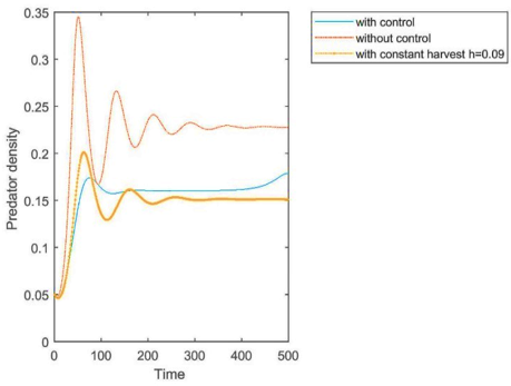
The initial conditions are (0.1, 0.05) with these set of values, we have the whole optimal amount of harvesting of Jopt=0.0363. Table 5 compares the whole optimal amount of harvesting and other total harvesting policies with applying the same values of the parameters. The optimal control variable, and the influence of the optimal harvesting on the prey and predator populations are indicated and shown in Figure 6 (a-c).
(a)
(b)
(c)
Figure 6. (a) Effecting of the optimal harvesting; (b) Effecting of the optimal harvesting for the prey populations; (c) Effecting of the optimal harvesting for the predator populations
Table 3. The parameter’s value for the fixed point e0, e1 and e2 for the discrete Model (5)
|
Parameter’s Value |
e0 |
e1 |
e2 |
|
r0 |
0.1 |
0.6 |
0.8 |
|
k |
0.3 |
0.3 |
0.7 |
|
d |
0.1 |
0.2 |
0.25 |
|
c |
0.1 |
0.1 |
0.4 |
|
h |
0.1 |
0.1 |
0.1 |
|
r |
0.5 |
0.4 |
0.7 |
|
a |
0.2 |
0.4 |
0.6 |
|
e |
0.1 |
0.3 |
0.5 |
|
f |
0.4 |
0.3 |
0.16 |
Table 4. Parameter’s value for optimal harvesting
|
Parameters |
Values |
|
r0 |
0.6 |
|
k |
0.4 |
|
d |
0.25 |
|
c |
0.5 |
|
h |
h* |
|
r |
0.7 |
|
a |
0.7 |
|
e |
0.65 |
|
f |
0.16 |
Table 5. The whole optimal amount of harvesting with other harvesting policies
|
The Harvesting Strategy |
The Total Harvesting (J) |
|
ht=h* |
Jopt=0.0363 |
|
ht=0.084 |
J=0.0355 |
|
ht=0.078 |
J=0.0354 |
|
ht=0.086 |
J=0.0354 |
|
ht=0.088 |
J=0.0353 |
|
ht=0.076 |
J=0.0353 |
|
ht=0.090 |
J=0.0352 |
|
ht=0.07 |
J=0.0348 |
|
ht=0.10 |
J=0.0338 |
|
ht=0.06 |
J=0.0330 |
|
ht=0.2 |
J=-0.0393 |
In this article, the behaviors of a fractional-order predator-prey system is studied and discussed with fear effect on prey population and harvesting rate as well as discrete conformable fractional-order system. The impact of fear effect on prey population and harvesting rate into above systems are made these systems more realistic. The existence and uniqueness as well as the non-negativity and boundedness of the solutions to the considered system are shown. It is observed that the considered model has three equilibrium points. Moreover, sufficient conditions are set to ensure and confirm the local asymptotic stability of the equilibrium points of the system. For the fractional-order system, it is seen that all equilibrium points are locally stable under some conditions on the parameters, namely the growth rate, the fear parameter and others. Furthermore, the discrete system is extended to the optimal harvesting problem to obtain the optimal harvesting amount. It is found that the constant policy cannot be the optimal choice for management. Therefore, the constant rate harvesting does not allow the optimal profit at all, so that the optimal harvesting can also persevere the population far from the collapse. The problem is solved through the discrete of Pontryagin's maximum principle. Also, numerical simulation shows that the fear effect on prey and harvesting rate take important issues in maintaining the prey and predator species.
|
R2+ |
The real positive region in two dimensions |
|
|
Dq |
Caputo’s fractional derivative |
|
|
Eq |
Mittag-Liffler function for one parameter |
|
|
J |
The Jacobian matrix |
|
|
T |
The time horizon |
|
|
Ht |
Hamiltonian function |
|
|
J(h) |
The objective function |
|
[1] Yousif, M.A., Al-Husseiny, H.F. (2021). Stability analysis of a diseased prey-predator-scavenger system incorporating migration and competition. International Journal of Nonlinear Analysis and Applications, 12(2): 1827-1853. https://doi.org/10.22075/IJNAA.2021.5320
[2] Wang, X., Zanette, L., Zou, X. (2016). Modelling the fear effect in predator–prey interactions. Journal of Mathematical Biology, 73(5): 1179-1204. https://doi.org/10.1007/s00285-016-0989-1
[3] Zhang, H., Cai, Y., Fu, S., Wang, W. (2019). Impact of the fear effect in a prey-predator model incorporating a prey refuge. Applied Mathematics and Computation, 356: 328-337. https://doi.org/10.1016/j.amc.2019.03.034
[4] Cresswell, W. (2011). Predation in bird populations. Journal of Ornithology, 152(Suppl 1): 251-263. https://doi.org/10.1007/s10336-010-0638-1
[5] Xu, S. (2014). Dynamics of a general prey–predator model with prey-stage structure and diffusive effects. Computers & Mathematics with Applications, 68(3): 405-423. https://doi.org/10.1016/j.camwa.2014.06.016
[6] Lan, Y., Shi, J., Fang, H. (2022). Hopf bifurcation and control of a fractional-order delay stage structure prey-predator model with two fear effects and prey refuge. Symmetry, 14(7): 1408. https://doi.org/10.3390/sym14071408
[7] Samko, S.G., Kilbas, A.A., Marichev, O.I. (1993). Fractional Integrals and Derivatives. Gordon and Breach Science Publishers, Yverdon Yverdon-les-Bains, Switzerland.
[8] Miller, K.S., Ross, B. (1993). An Introduction to the Fractional Calculus and Fractional Differential Equations. New York, Jon Wiley & Sons.
[9] Kar, T.K., Ghosh, B. (2012). Sustainability and optimal control of an exploited prey predator system through provision of alternative food to predator. Biosystems, 109(2): 220-232. https://doi.org/10.1016/j.biosystems.2012.02.003
[10] Sujatha, K., Gunasekaran, M. (2016). Dynamics in a harvested prey-predator model with susceptible-infected-susceptible (SIS) epidemic disease in the prey. Advances in Applied Mathematical Biosciences, 7(1): 23-31.
[11] Ahmed, R. (2020). Complex dynamics of a fractional-order predator-prey interaction with harvesting. Open Journal of Discrete Applied Mathematics, 3(3): 24-32.
[12] Al-Momen, S., Naji, R.K. (2022). The dynamics of modified Leslie-Gower predator-prey model under the influence of nonlinear harvesting and fear effect. Iraqi Journal of Science, 63: 259-282.
[13] Gorenflo, R., Mainardi, F, Podlubny, I. (1999). Fractional Differential Equations. Acad. Press, 8: 683-699.
[14] Li, H.L., Zhang, L., Hu, C., Jiang, Y.L., Teng, Z. (2017). Dynamical analysis of a fractional-order predator-prey model incorporating a prey refuge. Journal of Applied Mathematics and Computing, 54: 435-449. https://doi.org/10.1007/s12190-016-1017-8
[15] Mahdi, W.A.A., Al-Nassir, S. (2022). Dynamical behaviours of stage-structured fractional-order prey-predator model with Crowley–martin functional response. International Journal of Differential Equations, 2022: 6818454. https://doi.org/10.1155/2022/6818454
[16] Rivero, M., Trujillo, J.J., Vázquez, L., Velasco, M.P. (2011). Fractional dynamics of populations. Applied Mathematics and Computation, 218(3): 1089-1095. https://doi.org/10.1016/j.amc.2011.03.017
[17] Liu, X., Xiao, D. (2007). Complex dynamic behaviors of a discrete-time predator–prey system. Chaos, Solitons & Fractals, 32(1): 80-94. https://doi.org/10.1016/j.chaos.2005.10.081
[18] Chen, F. (2008). Permanence in a discrete Lotka–Volterra competition model with deviating arguments. Nonlinear Analysis: Real World Applications, 9(5): 2150-2155. https://doi.org/10.1016/j.nonrwa.2007.07.001
[19] El Raheem, Z.F., Salman, S.M. (2014). On a discretization process of fractional-order logistic differential equation. Journal of the Egyptian Mathematical Society, 22(3): 407-412. https://doi.org/10.1016/j.joems.2013.09.001
[20] Shafeii Lashkarian, R., Behmardi Sharifabad, D. (2018). Discretization of a fractional order ratio-dependent functional response predator-prey model, bifurcation and chaos. Computational Methods for Differential Equations, 6(2): 248-265.
[21] Shalsh, O.K., Al-Nassir, S. (2020). Dynamics and optimal harvesting strategy for biological models with Beverton-Holt growth. Iraqi Journal of Science, 223: 232.
[22] Holling, C.S. (1959). The components of predation as revealed by a study of small-mammal predation of the European Pine Sawfly1. The Canadian Entomologist, 91(5): 293-320.
[23] Holling, C.S. (1959). Some characteristics of simple types of predation and parasitism1. The Canadian Entomologist, 91(7): 385-398. https://doi.org/10.4039/Ent91385-7
[24] Dai, F., Feng, X., Li, C. (2014). Existence of coexistent solution and its stability of predator-prey with Monod-Haldane functional response. Journal of Xi’an Technological University, 34(11): 861-865.
[25] Andrews, J.F. (1968). A mathematical model for the continuous culture of microorganisms utilizing inhibitory substrates. Biotechnology and Bioengineering, 10(6): 707-723. https://doi.org/10.1002/bit.260100602
[26] Odibat, Z.M., Shawagfeh, N.T. (2007). Generalized Taylor’s formula. Applied Mathematics and Computation, 186(1): 286-293. https://doi.org/10.1016/j.amc.2006.07.102
[27] Ahmed, E., El-Sayed, A.M.A., El-Saka, H.A. (2006). On some Routh–Hurwitz conditions for fractional order differential equations and their applications in Lorenz, Rössler, Chua and Chen systems. Physics Letters A, 358(1): 1-4. https://doi.org/10.1016/j.physleta.2006.04.087
[28] Al-Nassir, S. (2021). Dynamic analysis of a harvested fractional-order biological system with its discretization. Chaos, Solitons & Fractals, 152: 111308. https://doi.org/10.1016/j.chaos.2021.111308
[29] Elsadany, A.A., Matouk, A.E. (2015). Dynamical behaviors of fractional-order Lotka–Volterra predator–prey model and its discretization. Journal of Applied Mathematics and Computing, 49: 269-283. https://doi.org/10.1007/s12190-014-0838-6
[30] Al-Nassir, S. (2021). The dynamics of biological models with optimal harvesting. Iraqi Journal of Science, 3039-3051.
[31] Al-Nassir, S. (2022). Optimal harvesting strategy of a discretization fractional-order biological model. Iraqi Journal of Science, 4957-4966. https://doi.org/10.24996/ijs.2022.63.11.32
[32] Gamkrelidze, R.V., Pontrjagin, L.S., Boltjanskij, V.G. (1964). The Mathematical Theory of Optimal Processes. Macmillan Company.
[33] Lenhart, S., Workman, J.T. (2007). Optimal Control Applied to Biological Models. Chapman and Hall/CRC.