Rafi M. Qasim![]() | Ihsan A. Abdulhussein
| Ihsan A. Abdulhussein![]() | Saja M. Naeem*
| Saja M. Naeem*![]() | Qusay A. Maatooq
| Qusay A. Maatooq![]()
© 2024 The authors. This article is published by IIETA and is licensed under the CC BY 4.0 license (http://creativecommons.org/licenses/by/4.0/).
OPEN ACCESS
This paper investigates experimentally the changing of a hydraulic characteristic of combined hydraulic structure owing to the existence of dike structure. Different models of combined structures are used with rectangular gates and rectangular weirs, respectively. Also, the location of the dike structure is considered. A dike is located upstream, downstream, and on both sides of the combined hydraulic structure. Discharge quantity, average downstream water depth, discharge coefficient, and Reynolds number are adopted to describe the alteration in hydraulic behavior of a combined structure. While the relation between upstream Froude number and downstream Froude number, as well as the relation between downstream Froude number with distance, are employed to illustrate the interactive response between dike and combined structure, From the study, the relation between Froude number at downstream and non-dimensional downstream distance as well as the relation between non-dimensional downstream water depth and non-dimensional distance reveal how the dike location effects on water depth and flow velocity, which lead to a change in the type of flow. Here, the dike position is shared in the form of a hydraulic jump at downstream of the combined structure. The experimental data were statistically analyzed to ensure their validity and reliability. The importance of this study is concentrated on how the location of the dike structure is shared in the alteration in the hydraulic characteristics of the combined hydraulic structure, especially the rise in the water depth at downstream, in addition to the change in the hydraulic jump height and energy losses.
combined discharge structure, dike, flow measurement, open channel flow
The combined hydraulic structure (discharge structure) comprises two different hydraulic structures: the first is called the weir, while the second is called the gate. Here, the combined structure does two different jobs at the same time; the first job is to remove the floating material by the weir, while the second job is to remove sediment material by the gate. The discharge structure has an important role in the management of the water quantity in an open channel, it is importance comes from the ability to measure the flow, divert the flow direction and prevent the problem of floating material and sediment material accumulation. While the dike structure has a vital role in reducing the flow turbulence and contributing to increasing the water depth. The existence of the combined hydraulic structure in the proximity of the dike structure refers to the fluid–structure–interaction where the alteration in the hydraulic response depends on both structures. Several researchers deal with both structures. Here, we mention some previous works. Qasim et al. [1], Quasim et al. [2], Qasim et al. [3] made many experimental studies to assess the hydraulic field at the downstream of the combined discharge structure under the action of the submerged obstacles. From the results they found that the obstacles have a major impact on the hydraulic characteristics of the discharge structure like actual discharge, discharge coefficient, downstream water flow velocity, and downstream water depth. Qasim et al. [4] did some experiments to assess the role of the combined discharge structure inclination angle in the alteration of the hydraulic structure characteristics. The inclination angle refers to the angle between the combined hydraulic structure and the horizontal bed of the flume. Qasim et al. [5] did some experiments to study the influence of the bed flume contraction on the combined structure discharge coefficient, also this work also dealt with Reynolds number, Froude number, actual discharge, flow velocity and downstream water depth. Yossef and de Vriend [6] performed experimental investigation in order to study the flow pattern for both submerged and emergent groynes. The groynes are installed in one side of straight fixed bed flume. The measurements show the changes in the nature of the turbulence between emerged and submerged groynes and give insight into the flow pattern in the proximity of groynes, also the study dealt with mixing layer shape and extent, and the flow velocity dynamic behavior. Yazdi et al. [7] used a numerical model to study the flow field around a groyne (a single dike). Three-dimensional flow is adopted. The study dealt with the reattachment length for various cases, distribution of the bed shear stress, flow rate, the angle and the length of the dike. Yaeger and Duan [8] studied numerically the flow field around a series of dikes in a fixed bed channel. The study concentrated on the Reynolds stresses and the turbulence intensities. Haltigin et al. [9] investigated numerically and experimentally the flow pattern around a deflector. A three-dimensional numerical model is employed in order to simulate the flow pattern around a deflector in a laboratory flume. Predicted velocities were successfully evaluated against laboratory measurements. Ettema and Muste [10] investigated a series of laboratory experiments and obtained scale influences in the small-scale models of the flow around a single dike installed in a channel with flat and fixed bed. Zeinivand et al. [11] performed an experimental test to show the effect of gate numbers and dimensions on the composite weir-gate discharge coefficient. The results lead to an increase in discharge coefficient with an increase in the number and dimensions of gates. Nouri et al. [12] used computational fluid dynamics to estimate the discharge coefficient of a composite compound rectangular broad crest weir gate. Diwedar et al. [13] did an experimental test to investigate flow passing through a composite triangular weir-triangular gate that is fixed into a straight channel. Three different notch angles are used in this study for the weir. The aim of the paper was to concentrate on the effect of composite geometry, head upstream, and depth of tailwater on the composite discharge coefficient, conveyed discharge, and flow patterns downstream. Ahmadabadi and Vatani [14] used five different methods relying on artificial neural networks to assess the weir-gate discharge coefficient. Altan-Sakarys et al. [15] studied numerically two different problems: the first dealt with weir, while the second dealt with composite weir-gate. The paper concentrated on the comparison between the numerical investigations of the two different problems with experimental data.
The main target of the current paper is based on how the dike structure affects the hydraulic characteristics of the combined discharge structure. Additionally, is it the dike structure that is more significant in sharing the hydraulic characteristics of the discharge structure? To this end, an experimental investigation is performed in a fixed and flat-bed flume containing a dike on both sides. The present experimental study seeks to investigate the impact of the dike on the combined hydraulic structure, where the dike is placed upstream of the combined structure, downstream of the combined structure, and on both sides of the combined structure. Also, a statistical analysis is performed to support the experimental results. The main parameters adopted in this study are the actual flow rate, average downstream water depth, discharge coefficient, Froude number, and Reynolds number. In addition, hydraulic jump height and energy losses are calculated for different cases.
2.1 Hydraulic characteristics concepts
The flow through the combined discharge structure can be expressed as the summation of the flow that crosses the weir and the gate. The flow rate can be calculated as shown below.
For weir: The theoretical discharge which crosses the rectangular weir can be computed from the equation [16]:
$Q_w=\frac{2}{3} \sqrt{2 g} b h^{3 / 2}$ (1)
For gates, the theoretical discharge that crosses the gate can be calculated using:
$Q_g=V A=\sqrt{2 g H} A$ (2)
From Eq. (2), it is evident that the theoretical velocity is expressed as a function of the channel upstream water depth [17-19]. With regard to the free flow:
$H=d+y+h$ (3)
With regard to the submerged flow:
$H=d+y+h-h_d$ (4)
With regard to the combined discharge structure.
The actual the theoretical discharge can be computed from:
$Q_{\text {theo }}=Q_w+Q_g$ (5)
$Q_{\text {act }}=c_d Q_{\text {theo }}$ (6)
$Q_{a c t}=c_d\left[Q_w+Q_g\right]$ (7)
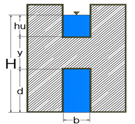
where, H: Upstream water depth, h represents the water head over the weir, y represents the vertical distance between the weir and the gate, d represents the gate depth. A: flow cross sectional area that crosses the gate, V: flow velocity, b: weir width, g: acceleration due to gravity, Qw: weir discharge, Qg: gate discharge, Qtheor: theoretical discharge, Qact: actual discharge, cd: Discharge coefficient.
Eqs. (1) to (4) include hydraulic and geometrical variables that dominate the hydraulic response of the combined structure. Here, it must be mentioned that the geometrical variable appears clearly in Eqs. (3) and (4); it is expressed by (y), where it refers to the vertical distance between the weir and gate. Froude Number [20] also Reynolds Number [21] are computed by using the equations:
$F_r=\frac{V}{\sqrt{g y}}$ (8)
$R_e=\frac{V h_d}{v}$ (9)
where, ν is water kinematic viscosity.
Both the Froude number and Reynolds number represent remarkable non-dimensional parameters to describe the type of flow, especially the Froude number, which is an important parameter in open channel flow. Hydraulic jump occurs when flow type change from supercritical to subcritical [22] hydraulic jump height is referred to the different between the depths after and before the jump [22].
$h_j=y_2-y_1$ (10)
The energy loss is expressed as [22]:
$\Delta E=\frac{\left(y_2-y_1\right)^2}{4 y_1 y_2}$ (11)
where, y2: Water depth after jump, y1: water depth before jump.
2.2 Experiments setup
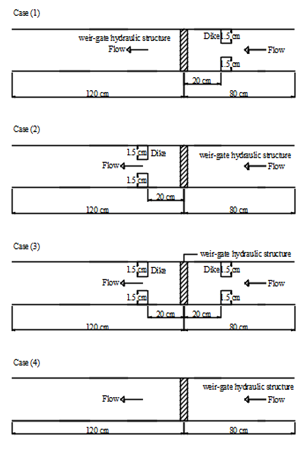
The experiments are performed in a flume with the following dimensions (200 cm length, 7.5 cm width and 15 cm depth). The combined discharge structure consists of two parts: the first part is the weir, and the second part is the gate. The study adopted different dimensions for the weir and gate. Table 1 outlines the dimensions of some selected combined discharge structures. The dike structure has a depth of 15cm and a width of 1.5cm. Both the combined discharge structure and the dike are made by using wood sheet material with a thickness of 5 mm. The volume method is employed to measure the actual flow rate (actual discharge), and the water depth is measured by using a scale fixed at the side wall of the flume. The measurements that are included in this study are the upstream water depth, downstream water depth, weir water head and actual discharge. Figure 1 shows the details of the combined discharge structure, and Figure 2 shows the hydraulic system, which consists of two parts: the dike structure and the combined discharge structure. The present paper deals with four different cases, and these cases are:
Case 1: The dike structure is installed at the upstream zone of the combined discharge structure.
Case 2: The dike structure is installed at the downstream zone of the combined discharge structure.
Case 3: The dike structure is installed in both zones (upstream and downstream).
Case 4: There is no dike structure in the flume.
Table 1. The composite structure models details
|
Model No. |
hu (cm) |
y (cm) |
d (cm) |
b (cm) |
H (cm) |
Aw (cm2) |
Ag (cm2) |
|
1 |
3 |
3 |
4 |
2 |
10 |
6 |
8 |
|
2 |
2 |
3 |
4 |
2 |
9 |
4 |
8 |
|
3 |
1 |
3 |
4 |
2 |
8 |
2 |
8 |
|
4 |
4 |
3 |
3 |
2 |
10 |
8 |
6 |
|
5 |
3 |
3 |
3 |
2 |
9 |
6 |
6 |
|
6 |
2 |
3 |
3 |
2 |
8 |
4 |
6 |
|
7 |
1 |
3 |
3 |
2 |
7 |
2 |
6 |
|
8 |
4 |
2 |
4 |
3 |
10 |
12 |
12 |
|
9 |
3 |
2 |
4 |
3 |
9 |
9 |
12 |
|
10 |
2 |
2 |
4 |
3 |
8 |
6 |
12 |
|
11 |
1 |
2 |
4 |
3 |
7 |
3 |
12 |
|
12 |
4 |
4 |
2 |
3 |
10 |
12 |
6 |
|
13 |
2 |
4 |
2 |
3 |
8 |
6 |
6 |
|
14 |
3 |
4 |
2 |
3 |
9 |
9 |
6 |
|
15 |
1 |
4 |
2 |
3 |
7 |
3 |
6 |
|
16 |
2 |
4 |
4 |
3 |
10 |
6 |
12 |
|
17 |
1 |
4 |
4 |
3 |
9 |
3 |
12 |
|
18 |
3 |
2 |
4 |
2 |
9 |
6 |
8 |
|
19 |
2 |
2 |
4 |
2 |
8 |
4 |
8 |
|
20 |
1 |
2 |
4 |
2 |
7 |
2 |
8 |
|
21 |
4 |
4 |
2 |
2 |
10 |
8 |
4 |
|
22 |
3 |
4 |
2 |
2 |
9 |
6 |
4 |
|
23 |
2 |
4 |
2 |
2 |
8 |
4 |
4 |
|
24 |
1 |
4 |
2 |
2 |
7 |
2 |
4 |
|
25 |
2 |
4 |
4 |
2 |
10 |
4 |
8 |
|
26 |
1 |
4 |
4 |
2 |
9 |
2 |
8 |
|
27 |
4 |
2 |
4 |
2 |
10 |
8 |
8 |
For all cases, the combined discharge structure is placed at a distance equal to 80 cm from the beginning of the flume. The bed of the flume is considered flat and fixed.
For case 1, the dike placement is at a distance equal to 20 cm upstream of the combined structure, while for case 2, the dike placement is at a distance equal to 20 cm downstream of the combined structure. Also, for case 3, the dike placement is at a distance equal to 20 cm on both sides of the combined structure. The dike is placed perpendicular to the bed of the flume to make a right angle with the flume wall on both sides of the dike.
Figure 1. Detail of the combined discharge structure
Figure 2. The dike structure and the combined discharge structure
The interaction between the dike structure and the composite weir-gate structure is a very important matter in the river system operation owing to the change in the hydraulic characteristics of weir-gate structure under the action of the dike structure, therefore this paper deal with this issue to give some image about this hydraulic interaction. Tables 2, 3, and 4 include the measured actual discharge, the average downstream water depth, and the calculated Reynolds number for different discharge structure models, respectively. For Table 2, computation shows six models with maximum discharge in case 1, four models with maximum discharge in case 2, five models with maximum discharge in case 3, and nine models with maximum discharge in case 4. It is obvious that case 4 usually produces the maximum actual discharge as compared with the remainder of the cases. This happens because of the water flow without any confinement of the stream flow by the dike structure. Table 2 includes statistical data such as minimum, maximum, standard deviation, average, and skewness. It is clear that the range of the maximum value is between 0.5 and 0.5929, while the standard deviation is between 0.095 and 0.1061 and the average value is between 0.3030 and 0.3357 for different cases, respectively. There is a slightly variation in the values of maximum value, standard deviation, and average value. Skewness refers to the symmetry or distortion that deviates from the normal distribution. if the curve is shifted to the right or to the left, it is said to be skewed. The skewness of normal distribution is equal to zero. Skewness may be positive or negative. The positive skewness means that the curve is shifted to the right and the mean of the measured data is greater than the median, while the negative skewness means that the curve is shifted to the left and the mean of the measured data is less than the median. From Table 2, case 2 data obey the normal distribution, while the remainder of cases is approximately near the normal distribution.
Table 2. Actual discharge for different models
|
Model No. |
Qact. (l/s) |
|||
|
Case1 |
Case2 |
Case3 |
Case4 |
|
|
1 |
0.3846 |
0.3597 |
0.2991 |
0.3593 |
|
2 |
0.3055 |
0.3125 |
0.2553 |
0.2632 |
|
3 |
0.3096 |
0.2165 |
0.2313 |
0.2500 |
|
4 |
0.3704 |
0.3344 |
0.3067 |
0.5155 |
|
5 |
0.2885 |
0.2646 |
0.2611 |
0.3333 |
|
6 |
0.2439 |
0.2041 |
0.2381 |
0.2494 |
|
7 |
0.1638 |
0.1751 |
0.2101 |
0.1739 |
|
8 |
0.5848 |
0.5000 |
0.5929 |
0.5319 |
|
9 |
0.4695 |
0.4348 |
0.4673 |
0.5000 |
|
10 |
0.3155 |
0.3509 |
0.3390 |
0.4098 |
|
11 |
0.2747 |
0.3333 |
0.3226 |
0.3185 |
|
12 |
0.3846 |
0.4000 |
0.4348 |
0.3876 |
|
13 |
0.3704 |
0.3021 |
0.3774 |
0.3333 |
|
14 |
0.3333 |
0.2268 |
0.2703 |
0.3542 |
|
15 |
0.3021 |
0.1650 |
0.1767 |
0.2208 |
|
16 |
0.5263 |
0.4525 |
0.4902 |
0.4525 |
|
17 |
0.4854 |
0.3571 |
0.3571 |
0.4785 |
|
18 |
0.3344 |
0.3571 |
0.3448 |
0.3165 |
|
19 |
0.2770 |
0.3003 |
0.2899 |
0.3175 |
|
20 |
0.2519 |
0.2247 |
0.2037 |
0.2342 |
|
21 |
0.4630 |
0.2899 |
0.2419 |
|
|
22 |
0.2058 |
0.2500 |
0.2146 |
0.3333 |
|
23 |
0.1887 |
0.2016 |
0.2020 |
0.2151 |
|
24 |
0.1563 |
0.1149 |
0.1923 |
0.1592 |
|
25 |
0.3390 |
0.3333 |
0.3058 |
|
|
26 |
0.3226 |
0.2857 |
0.2469 |
|
|
27 |
0.3846 |
0.4348 |
0.3610 |
0.3497 |
|
Min= |
0.1563 |
0.1149 |
0.1767 |
0.1592 |
|
Max= |
0.5848 |
0.5000 |
0.5929 |
0.5319 |
|
Stdev= |
0.1061 |
0.0950 |
0.1009 |
0.1058 |
|
Average= |
0.3347 |
0.3030 |
0.3049 |
0.3357 |
|
Skewness= |
0.4627 |
0.0964 |
1.1664 |
0.2858 |
For Table 3, computation shows there is no model with maximum discharge in case 1, twelve models with maximum discharge in case 2, twelve models with maximum discharge in case 3, and two models with maximum discharge in case 4. It is obvious, that cases 2 and 3 usually produce the maximum average downstream water depth as compared with the remainder of the cases. This occurs owing to the presence of the dike structure, which leads to a rise the water depth in the downstream region. Table 3 includes statistical data such as minimum, maximum, standard deviation, average, and skewness. From Table 3, case 2 data obeys the normal distribution, while cases 1 and 3 have positive skewness, and case 4 has negative skewness.
Table 3. Average downstream water depth for different models
|
Model No. |
Haverge (cm) |
|||
|
Case1 |
Case2 |
Case3 |
Case4 |
|
|
1 |
2.41 |
3.91 |
3.88 |
2.59 |
|
2 |
2.77 |
3.58 |
3.58 |
2.79 |
|
3 |
2.89 |
2.95 |
3.16 |
2.57 |
|
4 |
2.85 |
3.89 |
4.03 |
2.08 |
|
5 |
2.86 |
3.19 |
3.38 |
3.54 |
|
6 |
2.62 |
3.04 |
3.09 |
3.01 |
|
7 |
2.52 |
2.87 |
3.17 |
2.56 |
|
8 |
2.72 |
5.25 |
5.1 |
2.46 |
|
9 |
2.69 |
4.73 |
4.87 |
2.84 |
|
10 |
2.83 |
4.51 |
3.95 |
3.52 |
|
11 |
3.41 |
3.72 |
3.71 |
3.64 |
|
12 |
2.87 |
4.52 |
4.92 |
2.96 |
|
13 |
2.45 |
3.88 |
3.92 |
3.51 |
|
14 |
2.77 |
3.29 |
3.51 |
3.34 |
|
15 |
2.58 |
2.98 |
2.56 |
2.77 |
|
16 |
2.15 |
4.63 |
4.85 |
3.96 |
|
17 |
2.11 |
4.12 |
3.89 |
1.53 |
|
18 |
2.2 |
4.09 |
3.85 |
2.70 |
|
19 |
3.23 |
3.6 |
3.35 |
3.21 |
|
20 |
2.99 |
3.21 |
2.71 |
2.83 |
|
21 |
4.18 |
4.2 |
3.32 |
|
|
22 |
2.86 |
3.31 |
2.82 |
3.31 |
|
23 |
2.74 |
2.83 |
2.99 |
2.68 |
|
24 |
2.42 |
2.39 |
2.69 |
2.29 |
|
25 |
1.99 |
4.41 |
3.63 |
|
|
26 |
1.79 |
4.1 |
3.76 |
|
|
27 |
2.73 |
4.7 |
4.1 |
3.80 |
|
Min= |
1.7900 |
2.3900 |
2.5600 |
1.5300 |
|
Max= |
4.1800 |
5.2500 |
5.1000 |
3.9600 |
|
Stdev= |
0.4697 |
0.7176 |
0.6938 |
0.5767 |
|
Average= |
2.6900 |
3.7741 |
3.6589 |
2.9371 |
|
Skewness= |
0.9192 |
0.0537 |
0.5194 |
-0.2910 |
For Table 4, computation shows seven models with maximum discharge in case 1, four models with maximum discharge in case 2, five models with maximum discharge in case 3, and nine models with maximum discharge in case 4. In all cases, the type of flow is considered turbulent. Table 4 includes statistical data such as minimum, maximum, standard deviation, average, and skewness. It is evident from Table 4, case 2 data obeys the normal distribution, while cases 1, 3 and 4 have positive skewness.
Table 4. Reynolds number for different models
|
Model No. |
Rn |
|||
|
Case1 |
Case2 |
Case3 |
Case4 |
|
|
1 |
5128 |
4796 |
3988 |
4790 |
|
2 |
4073 |
4167 |
3404 |
3509 |
|
3 |
4128 |
2886 |
3084 |
3333 |
|
4 |
4938 |
4459 |
4090 |
6873 |
|
5 |
3846 |
3527 |
3481 |
4444 |
|
6 |
3252 |
2721 |
3175 |
3325 |
|
7 |
2185 |
2335 |
2801 |
2319 |
|
8 |
7797 |
6667 |
7905 |
7092 |
|
9 |
6260 |
5797 |
6231 |
6667 |
|
10 |
4206 |
4678 |
4520 |
5464 |
|
11 |
3663 |
4444 |
4301 |
4246 |
|
12 |
5128 |
5333 |
5797 |
5168 |
|
13 |
4938 |
4028 |
5031 |
4723 |
|
14 |
4444 |
3023 |
3604 |
4444 |
|
15 |
4028 |
2200 |
2356 |
2943 |
|
16 |
7018 |
6033 |
6536 |
6033 |
|
17 |
6472 |
4762 |
4762 |
6380 |
|
18 |
4459 |
4762 |
4598 |
4219 |
|
19 |
3693 |
4004 |
3865 |
4233 |
|
20 |
3359 |
2996 |
2716 |
3123 |
|
21 |
6173 |
3865 |
3226 |
|
|
22 |
2743 |
3333 |
2861 |
4444 |
|
23 |
2516 |
2688 |
2694 |
2867 |
|
24 |
2083 |
1533 |
2564 |
2123 |
|
25 |
4520 |
4444 |
4077 |
|
|
26 |
4301 |
3810 |
3292 |
|
|
27 |
5128 |
5797 |
4813 |
4662 |
|
Min= |
2083 |
1533 |
2356 |
2123 |
|
Max= |
7797 |
6667 |
7905 |
7092 |
|
Stdev= |
1415 |
1267 |
1346 |
1411 |
|
Average= |
4462 |
4040 |
4066 |
4476 |
|
Skewness= |
0.4627 |
0.0964 |
1.1664 |
0.2858 |
The reasons which lead to the variation in the results of the measured actual discharge, average downstream water depth, and calculated Reynolds number are: Interaction between overflow and underflow, variation in head over the weir of the discharge structure, variation in the cross-sectional area of flow passing through the gate (in all cases, the gate is full). The location of the dike structure reflects in the flow velocity magnitude, which is directly proportional to discharge and inversely proportional to average downstream water depth. For Table 5, computation shows seven models with maximum discharge coefficient in case 1, three models with maximum discharge coefficient in case 2, three models with maximum discharge coefficient in case 3, and eleven models with maximum discharge coefficient in case 4. In comparison to the other cases, case 4 frequently produces the highest discharge coefficient. This occurs as a result of the stream flow being unconstrained by the dike structure. The minimum, maximum, standard deviation, average, and skewness are all included in Table 5. It is clear that the range of the minimum value is between 0.18 and 0.213, while the average value is between 0.241 and 0.245 for different cases, respectively. There is a slight variation in the values of the minimum value and average value. Table 5 shows positive skewness.
Table 5. Discharge coefficient of different models
|
Cd |
||||
|
Model No. |
Case1 |
Case2 |
Case3 |
Case4 |
|
1 |
0.2694 |
0.2520 |
0.2095 |
0.2517 |
|
2 |
0.2484 |
0.2540 |
0.2076 |
0.2139 |
|
3 |
0.2917 |
0.2039 |
0.2179 |
0.2356 |
|
4 |
0.2821 |
0.2547 |
0.2336 |
0.3019 |
|
5 |
0.2612 |
0.2396 |
0.2365 |
0.2714 |
|
6 |
0.2655 |
0.2221 |
0.2592 |
0.2282 |
|
7 |
0.2150 |
0.2298 |
0.2756 |
0.2226 |
|
8 |
0.2447 |
0.2092 |
0.2481 |
0.2433 |
|
9 |
0.2285 |
0.2116 |
0.2274 |
0.2337 |
|
10 |
0.1799 |
0.2000 |
0.1933 |
0.2130 |
|
11 |
0.1838 |
0.2230 |
0.2158 |
0.2502 |
|
12 |
0.2483 |
0.2582 |
0.2807 |
0.2816 |
|
13 |
0.3695 |
0.2402 |
0.3001 |
0.3326 |
|
14 |
0.2651 |
0.2262 |
0.2697 |
0.2788 |
|
15 |
0.3816 |
0.2084 |
0.2232 |
0.2843 |
|
16 |
0.2725 |
0.2343 |
0.2538 |
0.2310 |
|
17 |
0.2884 |
0.2122 |
0.2122 |
0.2715 |
|
18 |
0.2441 |
0.2607 |
0.2517 |
0.2350 |
|
19 |
0.2369 |
0.2568 |
0.2479 |
0.3976 |
|
20 |
0.2527 |
0.2255 |
0.2044 |
0.3219 |
|
21 |
0.4483 |
0.2807 |
0.2343 |
|
|
22 |
0.2454 |
0.2982 |
0.2560 |
0.3017 |
|
23 |
0.2824 |
0.3017 |
0.3023 |
0.3926 |
|
24 |
0.2960 |
0.2178 |
0.3643 |
0.2343 |
|
25 |
0.2633 |
0.2589 |
0.2375 |
|
|
26 |
0.2875 |
0.2546 |
0.2200 |
|
|
27 |
0.2414 |
0.2729 |
0.2266 |
0.2195 |
|
Min= |
0.180 |
0.200 |
0.193 |
0.213 |
|
Max= |
0.448 |
0.302 |
0.364 |
0.398 |
|
Stdev= |
0.056 |
0.028 |
0.037 |
0.052 |
|
Average= |
0.270 |
0.241 |
0.245 |
0.269 |
|
Skewness= |
1.4849 |
0.5141 |
1.4332 |
1.2716 |
Figure 3 shows the relation between non-dimensional ratio (hd⁄B) and ratio(D⁄B), where hd represents the average downstream water depth, D represents the downstream distance of the flume measured from the discharge structure downstream, and B represents the water surface width at the downstream region. The plotted figure adopts three models; these models have different hydraulic and geometric variables. It is observed that, when the distance increases, the downstream water depth will decrease. This trend is common for the three models, and it happens owing to the friction losses that have grown and developed between water flow and the solid boundary and also the friction force between the water particles, which share shortages in the water depth at the downstream region. The effect of the dike structure on the water level is apparent clearly in the region when the ratio (D/B) is between 2 and 2.8 approximately. Here, in this position, the water depth will be raised owing to the intercept of the water flow by the dike structure. It is very important to concentrate on model 13, case 1. Here, the flow is near critical or supercritical and this will be reflected directly at the water depth, which also appears clearly as compared with other cases. Interference between the overflow velocity and underflow velocity will be considered in the determination of the water level.
Figure 3. The non-dimensional downstream water levels profile
Figure 4 shows the relation between the Froude number at the flume downstream and the ratio (D⁄B), where D represents the downstream distance of the flume measured from the discharge structure downstream and B represents the water surface width at the downstream region. The plotted figure adopts three models, these models have different hydraulic and geometric variables. It is evident from the figure that when the distance increases, the Froude number will be increased slightly. This occurs due to a decrease in the water depth in the downstream region. Also, when the water depth decreases, the Froude number will be increased owing to the inversely proportional between them. For model 5, especially case 1, the effect of the hydraulic jump is appeared clearly, and this happens owing to the presence of the dike structure, which leads to a change in flow type from supercritical to subcritical. Also, for model 13 case 1, the flow type is near critical flow when the ratio (D/B) is equal to 2. For all cases of model 20, there is no dramatic alteration in the relationship trend between the Froude number and the ration (D/B). Figure 5 illustrates the relationship between the Froude number and ratio (D/B), where D refers to the location where the Froude number is calculated and B refers to the width of the water surface. Figure 5 sketches for some selected models, considering the four different cases. Here, Ag is the cross-sectional area of flow that passes the gate, and d refers to the water depth at the gate openings. For model (9), which has Ag/BH = 0.1778 and d = 4cm, in case (1), the maximum value of Fr is 1.39 and maximum value of Fr is 1.18 in case (4), but the value of maximum Fr is 0.45 for both cases (2 and 3). It is visible from figure that the position of the maximum Froude number is located near the composite hydraulic structure, and this occurs for both cases 1 and 4, while for cases 2 and 3 the maximum Froude number is located approximately near the end of the flume. For model (18), which has Ag/BH=0.1185 and d=4cm. in case (1), the maximum value of Fr is 1.16 and the maximum value of Fr is 1.39 in case (4), but the value of maximum Fr is 0.38 for both cases (2 and 3). It is visible from the figure that the position of maximum Froude number is located near the composite hydraulic structure, and this occurs for both cases 1 and 4, while for cases 2 and 3, the maximum Froude number is located approximately near the end of the flume. It is obvious that both models have the same value of (d=4cm) but differ in Ag/BH. The alteration in trend will be attributed to the flow velocity and water depth. As the flow velocity increases, the Froude number will also increase due to the direct proportionality between them. As the water depth increases, the Froude number will decrease due to the inversely proportional relationship between them. For model (5), which has Ag/BH = 0.088 and d = 3cm. in case (1), the maximum value of Fr is 1.21 and the maximum value of Fr is 0.4 for all cases 2, 3, and 4. It is visible from the figure that the position of the maximum Froude number is located near the composite hydraulic structure, and this occurs for case 1 while for cases 2 , 3, and 4, the maximum Froude number is located approximately near the end of the flume. For model (22) which has Ag/BH=0.059 and d=2 cm. in case (4), the maximum value of Fr is 0.48 and the maximum values range from 0.25 to 0.35 for all cases 1, 2, and 3.
Figure 4. Downstream froude number profile
Figure 5. Relation between froude number and (D/B) ratio
Figure 6 shows the relationship between the downstream Froude number and the upstream Froude number. The relationship is nonlinear for different cases. The figure expresses the relation among critical, subcritical, and supercritical flow, respectively, and, in other words, shows the relation between inertia force and gravitational force. For the downstream region, the flow is subcritical, which means the gravity force is dominant, while in the upstream region, the change from subcritical to supercritical occurs. Here, at supercritical flow, the inertia force is dominant.
Figure 6. Upstream and downstream froude number profile
Table 6 shows the occurrence of hydraulic jumps will not be affected by the presence of the dike structure, but it depends mainly on the flow velocity in the downstream region of the composite hydraulic structure. This table is constructed based on model 18. The hydraulic jumps occurred in cases 1 and 4. The table also shows the energy losses that occurred due to the jump.
Table 6. Detail of hydraulic jump and energy loss form model 18
|
Case |
Y1 |
Fr1 |
Y2 |
Fr2 |
H.J |
∆E |
|
1 |
1.2 |
1.082 |
1.7 |
0.642 |
0.5 |
0.01532 |
|
2 |
4.7 |
0.149 |
5.7 |
0.111 |
1 |
0.00933 |
|
3 |
4.6 |
0.148 |
5.8 |
0.105 |
1.2 |
0.01619 |
|
4 |
1 |
1.347 |
1.6 |
0.665 |
0.6 |
0.03375 |
This study deals with interference between two different structures that are constructed in side channels, so the following noticeable points are found.
1. The presence of the dike structure will cause changes and fluctuations in discharge quantity, flow velocity, downstream water depth and discharge coefficient.
2. The skewness is a good indicator to show if the experimental data follows the normal distribution or diverges.
3. The downstream water depth decreases with increasing in the downstream distance while the fluctuation will be associated owing to occur of the hydraulic jump.
4. Froude number will be increased with the flume's horizontal distance, which happens owing to the reduction in water depth with an increase in distance.
5. The location of the maximum value and minimum value of the Froude number depends mainly on the location of the dike with respect to the composite hydraulic structure.
6. The profile of Froude number with distance reveals the comparison study between two different cases of flow: free flow and submerged flow.
7. It is very important to distinguish between the four different cases. Because of the location of the dike structure, major changes in hydraulic characteristics of the composite structure will occur especially in hydraulic interaction between weir discharge, and gate discharge, in addition to water depth on both sides of the composite structure.
8. Because the relationship between the upstream Froude number and downstream Froude number can be used to express the interactive response between the dike and composite hydraulic structure, it shows the dominating force that controls the hydraulic region.
9. The selection of the suitable case in determining the suitable position of the dike structure will be based mainly on the supply of a satisfactory quantity of flow rate.
Practical applications and recommendations:
It is recommended to place the dike structure near the combined structure in order to increase the water depth in the downstream region. The location of the dike must be decided based on many experimental studies to avoid any variation in the supply quantity of water in an open channel with distance. In the current investigation, two options give a suitable and reasonable location for the dike: in the first option, the dikes are placed on both sides of the combined structure, while in the second option, the dike is placed downstream of the combined structure.
[1] Qasim, R.M., Mohammed, A.A., Abdulhussein, I.A., Maatooq, Q.A. (2021). Experimental investigation of multi obstacles impact on weir-gate discharge structure. International Journal of Mechatronics and Applied Mechanics, (9): 76-84. https://doi.org/10.17683/ijomam/issue9.11
[2] Qasim, R.M., Abdulhussein, I.A., Al-Asadi, K. (2020). The effect of barrier on the hydraulic response of composite weir-gate structure. Archives of Civil Engineering, 66(4): 97-118. https://doi.org/10.24425/ace.2020.135211
[3] Qasim, R.M., Abdulhussein, I.A., Mohammed, A.A., Maatooq, Q.A. (2020). The effect of the obstacle on the hydraulic response of the composite hydraulic structure. Incas Bulletin, 12(3): 159-172. https://doi.org/10.13111/2066-8201.2020.12.3.13
[4] Qasim, R.M., Abdulhussein, I.A., Al-Asadi, K.H.A.L.I.D. (2020). Experimental study of composite inclined weir–gate hydraulic structure. Wseas Transactions on Fluid Mechanics, 15: 54-61. https://doi.org/10.37394/232013.2020.15.5
[5] Qasim, R.M., Abdulhussein, I.A., Maatooq, Q.A. (2019). Effect of bed flume contraction on discharge coefficient of composite weir-gate structure. International Journal of Science and Engineering Investigations (IJSEI), 8(87): 40-45.
[6] Yossef, M.F., de Vriend, H.J. (2011). Flow details near river groynes: Experimental investigation. Journal of Hydraulic Engineering, 137(5): 504-516. https://doi.org/10.1061/(asce)hy.1943-7900.0000326
[7] Yazdi, J., Sarkardeh, H., Azamathulla, H.M., Ghani, A.A. (2010). 3D simulation of flow around a single spur dike with free-surface flow. International Journal of River Basin Management, 8(1): 55-62. https://doi.org/10.1080/15715121003715107
[8] Yaeger, M., Duan, J.G. (2010). Mean flow and turbulence around two series of experimental dikes. In World Environmental and Water Resources Congress 2010: Challenges of Change, pp. 1692-1701. https://doi.org/10.1061/41114(371)178
[9] Haltigin, T.W., Biron, P.M., Lapointe, M.F. (2007). Three-dimensional numerical simulation of flow around stream deflectors: The effect of obstruction angle and length. Journal of Hydraulic Research, 45(2): 227-238. https://doi.org/10.1080/00221686.2007.10525038
[10] Ettema, R., Muste, M. (2004). Scale effects in flume experiments on flow around a spur dike in flatbed channel. Journal of Hydraulic Engineering, 130(7): 635-646. https://doi.org/10.1061/(ASCE)0733-9429(2004)130:7(635)
[11] Zeinivand, M., Barani, S., Ghomeshi, M. (2024). Investigating the process of changing the discharge coefficient of the flow passing through the combined structure of rectangular sharp-crested weir with multiple-gate. Ain Shams Engineering Journal. 15(2): 102418. https://doi.org/10.1016/j.asej.2023.102418
[12] Nouri, M., Sihag, P., Kisi, O., Hemmati, M., Shahid, S., Adnan, A.R. (2023). Prediction of discharge coefficient in compound broad-crested-weir-gate by supervised data mining techniques. Sustainability, 15(1): 433. https://doi.org/10.3390/su15010433
[13] Diwedar, A.I., Mamdouh, L., Ibrahim, M.M. (2022). Hydraulics of combined triangular sharp crested weir with inverted V-shape gate. Alexandria Engineering Journal, 61(10): 8249-8262. https://doi.org/10.1016/j.aej.2022.01.059
[14] Ahmadabadi, S.A., Vatani, A. (2022). A study of five types of ANN-based approaches to predict discharge coefficient of combined weir-gate. Journal of Hydraulic Structures, 8(4). https://doi.org/10.22055/jhs.2023.43234.1246
[15] Altan-Sakarys, A.B., Kokpinar, M.A., Duru, A. (2020). Numerical modelling of contracted sharp-crested weirs and combined weir and gate systems. Irrigation and Drainage, 69(4): 854-864. https://doi.org/10.1002/ird.2468
[16] Streeter, V.L., Wylie, E.B. (1983). Fluid mechanics. First SI Metric Edition.
[17] Rajaratnam, N., Subramanya, K. (1967). Flow equation for the sluice gate. Journal of the Irrigation and Drainage Division, 93(3): 167-186. https://doi.org/10.1061/JRCEA4.0000503
[18] Novak, P., Moffat, A.I.B., Nalluri, C., Narayanan, R.A.I.B. (2017). Hydraulic Structures. CRC Press.
[19] Swamee, P.K. (1992). Sluice-gate discharge equations. Journal of Irrigation and Drainage Engineering, 118(1): 56-60. https://doi.org/10.1061/(ASCE)0733-9437(1992)118:1(56)
[20] Fox, R.W., McDonald, A.T. (1994). Introduction to Fluid Mechanics. John Wiley and Sons, Inc.
[21] Negm, A.A.M., Al-Brahim, A.M., Alhamid, A.A. (2002). Combined-free flow over weirs and below gates. Journal of Hydraulic Research, 40(3): 359-365. https://doi.org/10.1080/00221680209499950
[22] Chow, V.T. (1983). Open-Channel Hydraulics. McGraw-Hill.