Vidhya Kannan![]() | Saraswathi Appasamy*
| Saraswathi Appasamy*![]()
© 2023 IIETA. This article is published by IIETA and is licensed under the CC BY 4.0 license (http://creativecommons.org/licenses/by/4.0/).
OPEN ACCESS
The realms of Intuitionistic Fuzzy Sets (IFSs), Pythagorean Fuzzy Sets (PFS), and q-rung Orthopair Fuzzy Sets (q-ROFSs) have found extensive applications across various disciplines, notably in resolving real-world problems. However, limitations concerning membership and non-membership grades pose challenges to these theories. Efforts to mitigate these constraints have led to the introduction of a new concept, the Linear Diophantine Fuzzy Set (LDFS), with reference parameters. This study advances the shortest path (SP) problem for Linear Diophantine Fuzzy graphs. An innovative method for constructing direct network graphs within a Linear Diophantine Fuzzy (LDF) context is proposed. Distances or costs between nodes are encapsulated by Linear Diophantine Fuzzy numbers. The principal contribution of this investigation lies in proposing a novel approach to solving the Linear Fuzzy Diophantine Fuzzy shortest path problem using the Bellman-Ford algorithm for optimal solution attainment. Usage of the score function enables the comparison and identification of the minimum arc value between nodes. The proposed algorithm's validity is demonstrated through a numerical example, and a comparison with existing methodologies underscores the benefits of the proposed algorithm.
shortest path problem, Bellman-Ford algorithm, score functions, Linear Diophantine Fuzzy arc weights, Linear Diophantine Fuzzy shortest path problem
The shortest path problem, an intriguing subject in operational research and graph theory, has been the focus of much scholarly attention. Researchers have developed numerous innovative approaches, algorithms, and models, all striving to find the optimal values—be they cost, time, or other considerations—that define the shortest path. Real-world complexities, such as varied weather conditions and traffic congestion, add layers of difficulty to these problems.
In 1965, Lotfi Zadeh introduced the concept of fuzzy set theory [1] to address these complexities. This theory expanded the traditional set theory to encapsulate fuzzy sets, which handle membership functions within a range of [0, 1]. Zadeh later proposed the concept of linguistic variables, whose values are expressed in natural language terms. When these words are articulated through fuzzy sets defined over a universal set, the variable is referred to as a fuzzy linguistic variable [2]. However, fuzzy sets only deal with membership functions.
To counter this limitation, Atanassov introduced an intuitionistic fuzzy set (IFS) [3], an extension of the fuzzy set where the total value of membership and non-membership does not exceed one. Further developments in this field led to the creation of the interval-valued intuitionistic fuzzy set (IVIFS) [4, 5], a generalization of the IFS. Despite their versatility, IFSs show limitations when the combined values of their membership and non-membership exceed one.
To address this, Yager proposed the Pythagorean fuzzy set (PyFS) [6-8], where the sum of the squared membership and non-membership values does not exceed one. Subsequently, Zhang and Xu [9, 10], Fei and Deng [11] and Peng and Ma [12] introduced ranking techniques for the order preference ideal solution and distance-based score methods for the Pythagorean fuzzy decision-making process. Garg and Rahman and Abdullah [13-17] proposed the interval-valued Pythagorean fuzzy set, a generalized form of PyFS, demonstrating its utility in decision-making processes through aggregation operators, Einstein operations, t-norms, and t-conorms.
Despite these advancements, the theories of IFS, PyFS, and q-ROFS have limitations in their membership and non-membership grades. To overcome this, several researchers [18-21] introduced the Linear Diophantine Fuzzy set (LDFS). Thanks to its unique ability to provide a broad characterization area for permissible doublets, the LDFS theory surpasses the IFS, PyFS, and q-ROFS theories in handling vague and uncertain information via reference parameters.
A comprehensive range of membership and non-membership grades in decision analysis is crucial for analyzing complex situations. The decision-maker has the flexibility to choose these degrees to incorporate reference factors. The LDFS, along with reference parameters, provides a reliable method for addressing modeling uncertainties, which encourages us to find the optimal path under LDFN.
The fuzzy shortest path problem (SPP) on a network was first addressed by Dubois [22]. Although they analyzed the shortest path, the shortest path corresponding to the distance no longer existed. Okada and Soper [23] and colleagues then introduced an algorithm for solving the SPP using the multiple labeling method for the multicriteria shortest path. Chuang and Kung [24, 25] proposed a novel algorithm where each arc length is represented as a triangular fuzzy set to find the fuzzy shortest path and fuzzy shortest path length. To address the shortcomings of existing algorithms, Deng et al. [26] employed the fuzzy Dijkstra algorithm to handle the SPP under uncertain environments. Numerous studies [27] have extended the Dijkstra algorithm to various fuzzy environments. Mukherjee [28] proposed a Dijkstra algorithm variation for the shortest path problem under intuitionistic fuzzy numbers. Kannan et al. [29] discussed the comparison between the fuzzy Floyd Warshall and fuzzy rectangular algorithms for the FSPP in their study. Kumar et al. [30] reviewed existing methods and proposed a fresh approach for the shortest path problem under a fuzzy environment.
A procedure [31] was developed for the shortest path problem on a network with fuzzy arc length named interval-valued fuzzy number matrices. Also, several approaches [32-40] were developed to evaluate the optimality of a variety of fuzzy theories for the fuzzy, intuitionistic fuzzy, and Pythagorean fuzzy shortest path problem. Broumi et al. [41] and Biswas et al. [42] conducted a literature survey on SPP under different fuzzy environments for various algorithms and identified the best methods for suitable conditions.
From the literature, it's evident that numerous algorithms exist for the study of the shortest path under various fuzzy environments. However, only limited work has incorporated reference parameters for SPP, motivating us to focus on the LDFN using the Bellman-Ford dynamic programming to find optimal solutions.
The Bellman-Ford method can handle graphs better than existing algorithms, particularly when certain edge weights are negative. It computes the shortest path in a graph with negative edges, reports the existence of a negative cycle, and aborts the computation of the undefined shortest path. This algorithm aims to provide the optimal fuzzy shortest path and the least LDF cost/time in a network-directed graph with LDF arc weights. The existing score function is used to compare the LDFNs and choose the minimum among them. A numerical example is provided to illustrate and discuss the efficiency and capabilities of the proposed method.
The contributions of this paper are:
In this section, the definitions of IFS, PyFS and LDFN, as well as some of their arithmetic and ranking operations are discussed.
Definition
An IFS $\mathfrak{J}$ on the universe $\mathfrak{Q}$ is defined by: $\mathfrak{J}=\{\mathfrak{x}, \mathfrak{m}(\mathfrak{x}), \mathfrak{n}(x), \mid \mathfrak{x} \in \mathfrak{Q}\}$ where $\mathfrak{m}: \mathfrak{Q} \rightarrow[0, 1]$ and $\mathfrak{y}: \mathfrak{Q} \longrightarrow[0, 1]$ represents the membership grade and non-membership grade of each $\mathfrak{x} \in \mathfrak{Q}$, respectively. A double set ($\mathfrak{m}, \mathfrak{n}$) is said to be IFS. Such that $0 \leq \mathfrak{m}(\mathrm{x})+\mathfrak{n}(\mathrm{x}) \leq 1$ for all $\mathfrak{x} \in \mathfrak{Q}$. Hesitation or indeterminacy part can be calculated as π($\mathfrak{x}$)=1−(σ($\mathfrak{x}$)+ρ($\mathfrak{x}$)). In some of the real-life scenarios IFS can’t work when σ($\mathfrak{x}$)+ρ($\mathfrak{x}$)>1 [6] named as PFS, which is also known as IFS type 2 by the study [3].
Definition [6]
A Pythagorean $\mathfrak{Q}_{\mathfrak{p}}$ fuzzy set (PyFS) on $\mathfrak{Q}$ is an object written as $\mathfrak{Q}_{\mathfrak{p}}=\left\{\left\langle \mathfrak{x}, \mathfrak{m}_{\mathfrak{p}}(\mathfrak{x}), \mathfrak{n}_{\mathfrak{p}}(\mathfrak{x})\right\rangle: \mathfrak{x} \in \mathfrak{Q}\right\}$ where $\mathfrak{m}_{\mathfrak{p}}(\mathfrak{x}) \in$ [0, 1] is the membership grade and $\mathfrak{y}_{\mathfrak{p}}(\mathfrak{x}) \in$ [0, 1] is the non-membership grade for each $\mathfrak{x}$ ∈ $\mathfrak{Q}$, respectively and the inequality $\mathfrak{m}_{\mathfrak{p}}^2(\mathfrak{x})+\mathfrak{n}_{\mathfrak{p}}^2(\mathfrak{x}) \leq 1$ holds for every $\mathfrak{x}$ ∈ $\mathfrak{Q}$. A double set ($\mathfrak{m}, \mathfrak{n}$) is said to be PyFS. The indeterminacy or hesitant part is calculated by $\pi_{\mathfrak{p}}(\mathfrak{x})=\sqrt{1-\mathfrak{m}_{\mathfrak{p}}^2(\mathfrak{x})-\mathfrak{n}_{\mathfrak{p}}^2(\mathfrak{x})}$.
Definition [21]
Let $\mathfrak{Q}$ be the non-reference set. A LDFS L on $\mathfrak{Q}$ is an object of the form $\mathfrak{L}_{\mathfrak{D}}=\left\{\left(\mathfrak{x},\left\langle\mathfrak{m}_{\mathfrak{D}}(\mathfrak{x}), \mathfrak{n}_{\mathfrak{D}}(x)\right\rangle ,\langle\alpha, \beta\rangle\right): \mathfrak{x} \in \mathfrak{Q}\right\} \mathfrak{L}_{\mathfrak{D}_2}$ where $\mathfrak{m}_{\mathfrak{D}}(\mathfrak{x}), \mathfrak{n}_{\mathfrak{D}}(\mathfrak{x})$ are the membership grade and non-membership grade respectively. Let $\alpha(\mathfrak{x}) \in[0,1]$ is the satisfaction grade reference parameter and $\beta(\mathfrak{x}) \in[0,1]$ is the dissatisfaction grade reference parameter. These grades satisfy the condition $0 \leq \alpha \mathfrak{m}_{\mathfrak{D}}(\mathfrak{x})+\beta \mathfrak{n}_{\mathfrak{D}}(\mathfrak{x}) \leq 1 \forall \mathfrak{x} \in \mathfrak{Q}$ with 0≤α+β≤1. These reference parameters can help in defining or classifying a particular system. By moving the physical meaning of these parameters, we can categorize the system. They expand the space used in LDFSs for grades and lift the limitation on them. The hesitation part can be evaluated as $\xi \pi_{\mathfrak{D}}=1-\left(\alpha \mathfrak{m}_{\mathfrak{D}}(\mathfrak{x})+\beta \mathfrak{n}_{\mathfrak{D}}(\mathfrak{x})\right)$, where ξ is the reference parameter related to degree of indeterminacy. The Linear Diophantine Fuzzy Number (LDFN) is defined as $\mathfrak{L}_{\mathfrak{D}}=\left(\left\langle\mathfrak{m}_{\mathfrak{D}}, \mathfrak{n}_{\mathfrak{D}}\right\rangle,\langle\alpha, \beta\rangle\right)$ with 0≤α+β≤1 and $0 \leq \alpha \mathrm{m}_{\mathfrak{D}}+\beta \mathfrak{n}_{\mathfrak{D}} \leq 1$. The space of IFS, PyFs, LDFS in shown in Figure 1.
Figure 1. Space of IFS, PyFs, LDFS
Definition [21]
A Linear Diophantine Fuzzy number (LDFN) can be written in the form of $\mathfrak{L}_{\mathfrak{D}}=\left(\left\langle\mathfrak{m}_{\mathfrak{D}}, \mathfrak{n}_{\mathfrak{D}}\right\rangle\left\langle\alpha_{\mathfrak{D}}, \beta_{\mathfrak{D}}\right\rangle\right)$ satisfy the following condition.
· $\mathfrak{m}_{\mathfrak{D}}, \mathfrak{n}_{\mathfrak{D}}, \alpha_{\mathfrak{D}} \beta_{\mathfrak{D}}$∈[0, 1]
·0≤$\alpha_{\mathfrak{D}}+\beta_{\mathfrak{D}}$≤1
·0≤$\mathfrak{m}_{\mathfrak{D}} \alpha_{\mathfrak{D}}+\mathfrak{n}_{\mathfrak{D}} \beta_{\mathfrak{D}}$≤1
Example: If $\mathfrak{m}_{\mathfrak{D}}$=0.89 and $\mathfrak{n}_{\mathfrak{D}}$=0.73, then 0.89+0.73=1.62$\not\leq$1 as well as (0.89)2+(0.73)2=1.325$\not\leq$1. However, with the arbitrary choice of parameter where α, β$\in$[0, 1] and 0≤α+β≤1 so that 0≤$\alpha \mathfrak{m}_{\mathfrak{D}}(\mathfrak{x})+\beta \mathfrak{n}_{\mathfrak{D}}(\mathfrak{x})$≤1. Let (α, β)=(0.55,0.49), therefore (0.89) (0.55)+(0.73) (0.49)=0.8472 <1. As a result, we were able to develop a more extensive space than the IFS and PyFS, and we now have additional alternatives for defining values to $\mathfrak{m}_{\mathfrak{D}}$ and $\mathfrak{n}_{\mathfrak{D}}$, which is not possible in the IFS and PyFS.
Definition [21]
A LDFS on $\mathfrak{Q}$ of the form 1 $\mathfrak{L}_{\mathfrak{D}}$={($\mathfrak{x}$,⟨1, 0⟩, ⟨1, 0⟩): $\mathfrak{x}$ ∈ $\mathfrak{Q}$} is called absolute LDFS and 0 $\mathfrak{L}_{\mathfrak{D}}$=($\mathfrak{x}$,⟨0, 1⟩,⟨0, 1⟩): $\mathfrak{x}$ ∈ $\mathfrak{Q}$} is called null or empty LDFS.
Definition [21]
Let $\mathfrak{L}_{\mathfrak{D}_i}=\left(\left\langle\mathfrak{m}_{\mathfrak{D}_i}, \mathfrak{n}_{\mathfrak{D}_i}\right\rangle,\left\langle\alpha_{\mathfrak{D}_i}, \beta_{\mathfrak{D}_i}\right\rangle\right)$ for i∈∆ be an assembling of LDFNs on $\mathfrak{Q}$ and $\mathfrak{X}>0$, then $\begin{aligned} & \mathfrak{L}_{\mathfrak{D}_1} \oplus \mathfrak{L}_{\mathfrak{D}_2}=\left(\left\langle\mathfrak{m}_{\mathfrak{D}_1}+\mathfrak{m}_{\mathfrak{D}_2}-\mathfrak{m}_{\mathfrak{D}_1} \mathfrak{m}_{\mathfrak{D}_2}, \mathfrak{n}_{\mathfrak{D}_1} \mathfrak{n}_{\mathfrak{D}_2}\right\rangle,\left\langle\alpha_{\mathfrak{D}_1}+\right.\right.\left.\left.\alpha_{\mathfrak{D}_2}-\alpha_{\mathfrak{D}_1} \alpha_{\mathfrak{D}_2}, \beta_{\mathfrak{D}_1} \beta_{\mathfrak{D}_2}\right\rangle\right)\end{aligned}$.
Definition [21]
Let $\mathfrak{L}_{\mathfrak{D}}$=(⟨$\mathfrak{m}_{\mathfrak{D}}$, $\mathfrak{n}_{\mathfrak{D}}$⟩,⟨α, β⟩) be an LDFN, then the score function (SF) is denoted by $\mathfrak{S}_{\left(\mathfrak{L}_{\mathfrak{D}}\right)}$ and the accuracy function (AF) by $\mathfrak{H}_{\left(\mathfrak{L}_{\mathfrak{D}}\right)}$ on D and can be defined by mapping $\mathfrak{S}$: LDFN$(\mathfrak{Q}) \rightarrow\lceil-1,-1\rceil$ and given by:
$\mathfrak{S}_{\left(\mathfrak{E}_{\mathfrak{D}}\right)}=\frac{1}{2}\left[\left(\mathfrak{m}_{\mathfrak{D}}-\mathfrak{n}_{\mathfrak{D}}\right)+(\alpha-\beta)\right]$ (1)
$\mathfrak{H}_{\left(\mathfrak{L}_{\mathfrak{D}}\right)}=\frac{1}{2}\left\lceil\frac{\left(\mathfrak{m}_{\mathfrak{D}}+\mathfrak{y}_{\mathfrak{D}}\right)}{2}+(\alpha+\beta)\right\rceil$ (2)
where, $\mathfrak{H}_{\left(\mathfrak{L}_{\mathfrak{D}}\right)}(\mathfrak{Q})$ is the assembling of all LDFNs on $\mathfrak{Q}$.
Definition [21]
If two LDFNs $\mathfrak{L}_{\mathfrak{D}_1}$ and $\mathfrak{L}_{\mathfrak{D}_2}$ can be comparable using the SF and the AF. This is defined as follows:
In this section, the mathematical formulation for Linear Diophantine Fuzzy shortest path is presented. Consider a graph $\mathfrak{G}=(\mathfrak{B}, \mathfrak{E})$ is an LDF-directed graph, where $\mathfrak{B}$={s=1, 2, ..., e =m} and $\mathfrak{B}$×$\mathfrak{B}$=$\mathfrak{G}$={(i, j): i, j∈$\mathfrak{B}$, i$\neq$j} denotes the vertex and edge set, respectively. The ordered pairs (i, j) represent the two different vertices that are connected by an edge of the graph i, j∈$\mathfrak{B}$. In a connected network, the arc source node s and destination node t. There is assumed to be only one path from node i to node j. The path $\mathfrak{p}$ij from node i to node j is a sequence of arcs $\mathfrak{p}$ij={(i, i1), (i1, i2), ......, (ik, j)} in which each arc’s initial node is same as the corresponding destination node. The problem is to identify the optimal path from node s to t for each arc-related parameter in terms of cost (or time, or distance, etc). In terms of LDFNs, this parameter is assumed to be $\mathfrak{c}_{\mathrm{ij}}=\left\langle\alpha_{\mathfrak{R}}(\mathfrak{ab}) \mathfrak{m}_{\mathfrak{R}}(\mathfrak{ab}) \beta_{\mathfrak{R}}(\mathfrak{ab}) \mathfrak{n}_{\mathfrak{R}}(\mathfrak{ab})\right\rangle$ where $\mathfrak{m}_{\mathfrak{R}}(\mathfrak{ab})$ is the membership grade and $\mathfrak{n}_{\mathfrak{R}}(\mathfrak{ab})$ is the non-membership grade and $\alpha_{\mathfrak{R}}(\mathfrak{ab})$, $\beta_{\mathfrak{R}}(\mathfrak{ab})$ are the reference parameters. The arc i-j represents the distance of the path in the shortest path problem. The main objective of the shortest path is to find the optimal path and minimum cost/distance/time from source node $\mathfrak{s}$ to the destination node t. Due to ambiguous situations, LDFN arc values are considered in the SP problem. Therefore, the resulting problem is called a Linear Diophantine Fuzzy shortest path problem (LDFSPP). The mathematical model of the problem is formulated as:
$\begin{aligned} & \operatorname{Min} \tilde{Z}=\sum_{i=1}^m \sum_{j=1}^m \tilde{c}^p x_{i j} \\ & \text { s.t } \sum_{j=1}^m x_{i j}-\sum_{k=1}^m x_{k i}=\left\{\begin{array}{cc}1 & i=1 \\ 0 & i \neq 1, m \\ -1 & i=m\end{array}\right. \\ & x_{i j} \geq 0, i, j=1,2 \ldots . m \\ & \end{aligned}$ (3)
If the arc (i, j) is in the path, then xij=1 else xij=0. Let Tst denote the set of all paths from node s to node t. Let $\widetilde{\mathfrak{E}}_{i j}^p$ be the Linear Diophantine Fuzzy cost of path from the node $\mathfrak{u}$ to node $\mathfrak{v}$.
3.1 The extended Bellman-Ford algorithm in Linear Diophantine Fuzzy environment
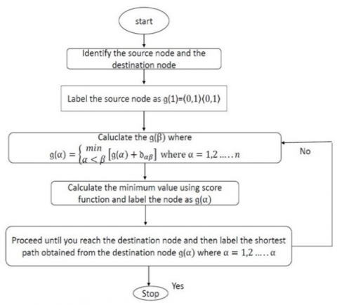
Let us consider acyclic-directed graph $\mathfrak{G}=(\mathfrak{B}, \mathfrak{E})$ from source node $\mathfrak{s}$ to the destination node $\mathfrak{t}$ with Linear Diophantine Fuzzy arc weights. The Bellman dynamic programming is used to determine the shortest path by the forward pass calculation. The Extended Bellman-Ford dynamic programming under Linear Diophantine Fuzzy environment is formulated as:
Initialization Step: Set the Source node as $\mathfrak{g}(1)=\langle 0,1\rangle\langle 0,1\rangle$ Main Step: $\min _{\alpha<\beta}\left[\mathfrak{g}(\alpha)+\mathfrak{d}_{\alpha \beta}\right]$ (4)
here, $\mathfrak{d}_{\alpha \beta}$ is the directed LDFN edge weight, $\mathfrak{g}(\alpha)$ is the LDFN arc length of the shortest path from the source node to destination node. The diagram illustrating the proposed model is depicted in Figure 2.
Theorem: If a LDF directed graph $\mathfrak{G}=(\mathfrak{B}, \mathfrak{E})$ contains no non-negative weight cycles then after Bellman-Ford completes execution $\mathfrak{d}[\mathfrak{v}]=\delta(\mathfrak{s}, \mathfrak{v})$ for all $\mathfrak{v} \in \mathfrak{B}$.
Proof: Let $\mathfrak{v} \in \mathfrak{B}$. If there is a path $\mathfrak{p}=\left\langle\mathfrak{v}_0, \mathfrak{v}_1 \ldots \ldots \ldots \mathfrak{v}_k\right\rangle$ then $\mathfrak{v}_0=\mathfrak{s}$ to $\mathfrak{v}_k=\mathfrak{B}$. Then a path $\mathfrak{p}$ is a simple path with minimum LDF number of edges. If there is no negative LDFN edge cycle then it implies $\mathfrak{p}$ is simple.
$\Rightarrow k \leq \mathfrak{d}[\mathfrak{v}]$.
After one visit through all the LDFN edges E, we have $\mathfrak{d}$$\left[\mathfrak{v}_1\right]=\delta\left(\mathfrak{s}, \mathfrak{v}_1\right)$ because the LDFN edge $\mathfrak{v}_0$, $\mathfrak{v}_1$ is relaxed. After the second visit through all the LDFN edges, we have $\mathfrak{d}$$\left[\mathfrak{v}_2\right]=\delta\left(\mathfrak{s}, \mathfrak{v}_2\right)$ because the LDFN edge ($\mathfrak{v}_1, \mathfrak{v}_2$). Similarly, after k visits, $\mathrm{d}\left[\mathfrak{v}_k\right]=\delta\left(\mathfrak{s}, \mathfrak{v}_k\right)$ which implies $|\mathfrak{B}|-1 \Longrightarrow$ all reachable vertex has δ values. Therefore, the Bellman-Ford executes d[v]=$\delta(\mathfrak{s}, \mathfrak{v})$ for all $\mathfrak{v} \in \mathfrak{B}$ when there are no non-negative weight cycles.
Corollary: If a value $\mathfrak{d}[\mathfrak{v}]$ fails to converge after |$\mathfrak{B}$|−1 visits there exists a negative LDFN weight cycle reachable from s because we will be able to relax the LDFN edge and reduce the LDFN weight after added vertex that form a cycle. Therefore, the cycle will be negative.
Proof: After |$\mathfrak{B}$|−1 visits. If there is an LDFN edge that can be relaxed. (i.e.) current shortest path from $\mathfrak{s}$ to some vertex $\mathfrak{v}$ which is reachable is not simple. Having repeated vertex, $\Rightarrow$then there exists a negative weight cycle.
Figure 2. Flow chart diagram representing the algorithm
|
Pseudocode for the proposed Linear Diophantine Fuzzy Bellman-Ford Algorithm (LDFBFA) |
|
1. Function Linear Diophantine Fuzzy Bellman-Ford Algorithm ($\mathfrak{G}$, $\mathfrak{s}$) 2. For each vertex $\mathfrak{B}$ ∈ $\mathfrak{G}$ do 3. $\mathfrak{d}[\mathfrak{v}] \leftarrow \infty$ 4. end for 5. $\mathfrak{d}[\mathfrak{s}] \leftarrow\langle 0,1\rangle\langle 0,1\rangle$ 6. for i$\leftarrow$1 to |$\mathfrak{v}$| do 7. relaxed$\leftarrow$false 8. for each (αβ) ∈ $\mathfrak{E}$ do 9. if $\mathfrak{g}[\alpha]$>$\mathfrak{g}[\beta]$+$\mathfrak{v}(\alpha, \beta)$ then 10. $\mathfrak{S}(\mathfrak{g}[\alpha]>\mathfrak{S}(\mathfrak{g}[\beta]+\mathfrak{d}(\alpha, \beta))$ do 11. $\mathfrak{g}[\alpha] \leftarrow \mathfrak{g}[\beta]+\mathfrak{d}(\alpha, \beta)$ 12. relaxed$\leftarrow$true 13. end if 14. end for 15. if relaxed=false then 16. exit the loop 17. end if 18. end for 19. for each (αβ) ∈ $\mathfrak{E}$ do 20. if $\mathfrak{S}(\mathfrak{g}[\alpha]<\mathfrak{S}(\mathfrak{g}[\beta]+\mathfrak{d}(\alpha, \beta))$ 21. return false 22. end if 23. end for 24. return true |
3.2 Numerical illustration
This section is based on adaptable numerical problem to illustrate the possible implementation of the proposed algorithm.
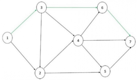
Example 1: Let us consider a disaster road network Figure 3, that occurred in Wenling City with Linear Diophantine Fuzzy distance discussed by the study [18]. The arc values for the network in terms of LDF Distance are shown in the Table 1.
Figure 3. The graph with Linear Diophantine Fuzzy distance
Table 1. Arc value in term of Linear Diophantine Fuzzy distance for Example 1
|
Edges |
LDFN |
Edges |
LDFN |
|
(1,2) |
(⟨0.81, 0.37⟩, ⟨0.51, 0.18⟩) |
(3,6) |
(⟨0.91, 0.73⟩, ⟨0.46, 0.18⟩) |
|
(1,3) |
(⟨0.93, 0.68⟩, ⟨0.53, 0.12⟩) |
(4,5) |
(⟨0.64, 0.29⟩, ⟨0.37, 0.28⟩) |
|
(2,4) |
(⟨0.74, 0.47⟩, ⟨0.43, 0.32⟩) |
(4,6) |
(⟨0.87, 0.39⟩, ⟨0.25, 0.22⟩) |
|
(2,5) |
(⟨0.93, 0.63⟩, ⟨0.46, 0.29⟩) |
(4,7) |
(⟨0.78, 0.57⟩, ⟨0.45, 0.21⟩) |
|
(3,2) |
(⟨0.94, 0.58⟩, ⟨0.58, 0.13⟩) |
(5,7) |
(⟨0.73, 0.68⟩, ⟨0.41, 0.37⟩) |
|
(3,4) |
(⟨0.64, 0.21⟩, ⟨0.37, 0.28⟩) |
(6,7) |
(⟨0.83, 0.43⟩, ⟨0.51, 0.15⟩) |
Iteration 1: Start from the source node. Let the $\mathfrak{g}(1)$=⟨0, 1⟩⟨0, 1⟩ and label $\mathfrak{g}(1)$=[⟨0, 1⟩⟨0, 1⟩, 1].
Iteration 2: Consider the node 1 as α and node 2 as β. Now relax the edges using Eq. (4). Using the score function [1] to choose the minimum one and label it as temporary node.
$\mathfrak{g}(2)=\min _{\alpha<2}\left[\mathfrak{~g}(\alpha)+\mathfrak{d}_{\alpha 2}\right]=\mathfrak{g}(1)$+$\mathfrak{d}_{12}=$⟨0, 1⟩⟨0, 1⟩+ ⟨0.81, 0.37⟩⟨0.51, 0.18⟩=⟨0.81, 0.37⟩⟨0.51, 0.18⟩$\mathfrak{G}$(⟨0.81, 0.37⟩⟨0.51, 0.18⟩)=0.385
Therefore, Label $\mathfrak{g}(2)$=[⟨0.81, 0.37⟩⟨0.51, 0.18⟩, 1→2]
Iteration 3: Repeat the process with the node 3 and relax all edges using the Eq. (4).
$\mathfrak{g}(3)=\min _{\alpha<3}\left[\mathfrak{~g}(\alpha)+\mathfrak{d}_{\alpha 3}\right]=\mathfrak{g}(1)$+$\mathfrak{d}_{13}=$⟨0, 1⟩⟨0, 1⟩+ ⟨0.93, 0.68⟩⟨0.53, 0.12⟩=⟨0.93, 0.68⟩⟨0.53, 0.12⟩
The score function 1 is used to identify the minimum one and label it as temporary node, $\mathfrak{G}$(⟨0.93, 0.68⟩⟨0.53, 0.12⟩)=0.33 and Label $\mathfrak{g}(3)$=[⟨0.93, 0.68⟩⟨0.53, 0.12⟩, 1→3]
Iteration 4: Repeat the same process for the node 4 and relax all the edges using the equation and using score function pick the minimum value and label it as temporary node.
$\mathfrak{g}(4)=\min_{\alpha<4}\left[\mathfrak{~g}(\alpha)+\mathfrak{d}_{\alpha 4}\right]=\min \left\{\mathfrak{g}(2)+\mathfrak{d}_{24}, \mathfrak{~g}(3)+\right. \left.\mathfrak{d}_{34}\right\}=\min \{\langle 0.81,0.37\rangle\langle 0.51,0.18\rangle+\langle 0.74,0.47\rangle\langle 0.43,0.32\rangle \text {, } \langle 0.93, 0.68\rangle\langle 0.53, 0.12\rangle+\langle 0.64, 0.21\rangle\langle 0.37, 0.28\rangle\}=\min \{\langle 0.9506,0.1739\rangle$
$\langle 0.7207,0.057\rangle,\langle 0.9748,0.1428\rangle\langle 0.7039 \text {, } 0.33\rangle\}$
Using Score Function 1, $\mathfrak{G}$(⟨0.9506, 0.1739⟩⟨0.7207, 0.057⟩)=0.7202$\mathfrak{G}$(⟨0.9748, 0.1428⟩⟨0.7039, 0.33⟩)=0.7514
Therefore, min{0.7202, 0.7514}=0.7202.
Hence label $\mathfrak{g}(4)$=[⟨0.9506, 0.1739⟩⟨0.7207, 0.057⟩, 1→2→4]
Iteration 5: Visit each edge that reaches the vertex 5 from the source node using the Eq. (4). Using the score function 1 pick the minimum one and label it as temporary vertex. Repeat this process for |$\mathfrak{B}$|−1 times.
$\mathfrak{g}(5)=\min_{\alpha<5}\left[\mathfrak{g}(\alpha)+\mathfrak{b}_{\alpha 5}\right]=\left\{\mathfrak{g}(2)+\mathfrak{b}_{25}, \mathfrak{g}(4)+\mathfrak{b}_{45}\right\}=\min\{\langle 0.81,0.37\rangle\langle 0.51,0.18\rangle+\langle 0.93,0.63\rangle\langle 0.46,0.29\rangle,\langle 0.9506, 0.1739\rangle\langle 0.7207,0.057\rangle+\langle 0.64,0.29\rangle\langle 0.37,0.28\rangle\}=\min\{\langle 0.9867,0.2233\rangle$
$\langle 0.7354,0.0522\rangle,\langle 0.982,0.0493\rangle\langle 0.8236, 0.0168\rangle\}$
Hence $\mathfrak{S}(\langle 0.9867,0.2233\rangle\langle 0.7354,0.0522\rangle)=0.7233$ $\mathfrak{S}(\langle 0.982,0.0493\rangle\langle 0.8236,0.0168\rangle)=0.8695$. Therefore, min{0.7233, 0.8695}=0.7233
The minimum node is chosen and labeled $\mathfrak{g}(5)=[\langle 0.9867$, $0.2233\rangle\langle 0.7354,0.0522\rangle, 1 \rightarrow 2 \rightarrow 5]$.
Iteration 6: Relax all edges that are reachable from the vertex 6 using the Eq. (4) and to fix the temporary node use the 1 score function.
$\mathfrak{g}(6)=\min_{\alpha<6}\left[\mathfrak{g}(\alpha)+\mathfrak{b}_{\alpha 6}\right]=\min\left\{\mathfrak{g}(3)+\mathfrak{b}_{36}, \mathfrak{g}(4)+\mathfrak{b}_{46}\right]$=min{⟨0.93, 0.68⟩⟨0.53, 0.12⟩+⟨0.91, 0.73⟩⟨0.46, 0.18⟩, ⟨0.9506, 0.1739⟩ ⟨0.7207, 0.057⟩+⟨0.97, 0.39⟩⟨0.25, 0.22⟩}=min{⟨0.9937, 0.4964⟩⟨0.7462, 0.0216⟩, ⟨0.9935, 0.0663⟩⟨0.79, 0.011⟩}
Hence $\mathfrak{G}$(⟨0.9937, 0.4964⟩⟨0.7462, 0.0216⟩)=0.61095(⟨0.9935, 0.0663⟩⟨0.79, 0.011⟩)=0.8536
Therefore, min {0.61095, 0.8536}=0.61095.
Hence, Label $\mathfrak{g}(6)$=[⟨0.9937, 0.4964⟩⟨0.7462, 0.0216⟩, 1→3→6]
Iteration 7: Visit all the edges that are reachable to the vertex 7(destination node) using 4 and use the score function to find the minimum value.
$\mathfrak{g}(7)=\min _{\alpha<7}\left[\mathfrak{~g}(\alpha)+\mathfrak{d}_{\alpha 7}\right]=\min \quad\left\{\mathfrak{g}(4)+\mathfrak{d}_{47}, \mathfrak{~g}(5)+\right.\left.\mathfrak{d}_{57}, \mathfrak{~g}(6)+\mathfrak{d}_{67}\right\}$=min{⟨0.9056, 0.1739⟩⟨0.7207, 0.057⟩+⟨0.78, 0.57⟩⟨0.45, 0.21⟩,⟨0.986, 0.223⟩⟨0.74, 0.052⟩+⟨0.73, 0.68⟩⟨0.41, 0.37⟩,⟨0.99, 0.49⟩⟨0.74, 0.22⟩+⟨0.83, 0.43⟩⟨0.51, 0.15⟩}=min {⟨0.989, 0.096⟩⟨0.846, 0.012⟩,⟨0.99, 0.149⟩ ⟨0.846, 0.018⟩,⟨0.998, 0.2107⟩⟨0.8726, 0.0003⟩}
Hence, $\mathfrak{S}$(⟨0.989, 0.096⟩⟨0.846, 0.012⟩)=0.8635 (⟨0.99, 0.149⟩⟨0.846, 0.018⟩)=0.834
$\mathfrak{S}$(⟨0.998, 0.2107⟩⟨0.8726, 0.0003⟩)=0.8301
Therefore, min {0.8635, 0.834, 0.8301}=0.8301
Therefore, choose the minimum node and Label $\mathfrak{g}(7)$=[⟨0.998, 0.2107⟩⟨0.8726, 0.0003⟩, 1→3→6→7]. The shortest path and the shortest distance using the proposed algorithm for the (Figure 1) are 1→3→6→7 and 0.8301 respectively. Figure 4 represents the optimal path using the proposed method. Table 2 represents the LDFN optimal values at each node using the proposed method.
Figure 4. The Shortest path of the network with Linear Diophantine Fuzzy distance using the proposed algorithm
Example 2: An example problem has been considered a wireless charging approach method for sensor networks as shown in Figure 5 from the study [40] for the proposed method. Table 3 presents the values of arcs expressed in terms of Linear Diophantine Fuzzy numbers for the network.
Table 2. The optimal value of LDFN at every node utilizing the proposed method in Example 1
|
Node α |
Shortest LDFN Path from Node 1 to α |
$\mathfrak{g}(α)$ |
|
2 |
1→2 |
⟨0.81, 0.37⟩⟨0.51, 0.18⟩ |
|
3 |
1→3 |
⟨0.93, 0.68⟩⟨0.53, 0.12⟩ |
|
4 |
1→2→4 |
⟨0.9506, 0.1739⟩⟨0.7207, 0.057⟩ |
|
5 |
1→2→5 |
⟨0.9867, 0.2233⟩⟨0.7354, 0.0522⟩ |
|
6 |
1→3→6 |
⟨0.9937, 0.4964⟩⟨0.7462, 0.0216⟩ |
|
7 |
1→3→6→7 |
⟨0.998, 0.2107⟩⟨0.8726, 0.0003⟩ |
Figure 5. The graph with Linear Diophantine Fuzzy distance
Table 3. Arc value in term of Linear Diophantine Fuzzy distance for Example 2
|
Edges |
LDFN |
|
(1,2) |
(⟨0.7, 0.6⟩, ⟨0.5, 0.3⟩) |
|
(1,4) |
(⟨0.4, 0.4⟩, ⟨0.6, 0.4⟩) |
|
(1,5) |
(⟨0.7, 0.8⟩, ⟨0.5, 0.3⟩) |
|
(2,3) |
(⟨0.9, 0.7⟩,⟨0.6, 0.2⟩) |
|
(2,4) |
(⟨0.6, 0.9⟩,⟨0.8, 0.2⟩) |
|
(3,4) |
(⟨0.8, 0.7⟩,⟨0.4, 0.3⟩) |
|
(3,6) |
(⟨0.8, 0.2⟩,⟨0.3, 0.2⟩) |
|
(4,5) |
(⟨0.9, 0.8⟩,⟨0.5, 0.3⟩) |
|
(4,6) |
(⟨0.6, 0.5⟩,⟨0.4, 0.1⟩) |
|
(4,7) |
(⟨0.8, 0.7⟩,⟨0.4, 0.3⟩) |
|
(5,7) |
(⟨0.8, 0.7⟩,⟨0.4, 0.3⟩) |
|
(5,8) |
(⟨0.9, 0.2⟩,⟨0.3, 0.1⟩) |
|
(6,7) |
(⟨0.4, 0.3⟩,⟨0.5, 0.3⟩) |
|
(7,8) |
(⟨0.9, 0.4⟩,⟨0.6, 0.4⟩) |
|
(6,10) |
(⟨0.7, 0.5⟩,⟨0.2, 0.1⟩) |
|
(8,9) |
(⟨0.3, 0.2⟩,⟨0.6, 0.4⟩) |
Iteration 1: Start from the source node.
Let the $\mathfrak{g}(1)$ and label $\mathfrak{g}(1)$=[⟨0, 1⟩⟨0, 1⟩, 1]
Iteration 2: Consider the node 1 as α and node 2 as β. Now relax the edges which reaches the node 2 using Eq. (4). Using the score function [1] to choose the minimum one and label it as temporary node.
$\mathfrak{g}(2)$=$\min_{\alpha<2}\left[\mathfrak{g}(\alpha)+\mathfrak{d}_{\alpha 2}\right]$=$\mathfrak{g}(1)+\mathfrak{b}_{12}$=⟨0, 1⟩⟨0, 1⟩+⟨0.7, 0.6⟩⟨0.5, 0.3⟩$\mathfrak{S}$⟨0.7, 0.6⟩⟨0.5, 0.3⟩(⟨0.7, 0.6⟩⟨0.5, 0.3⟩)=0.15.
Therefore, Label $\mathfrak{g}(2)$=[⟨0.7, 0.6⟩⟨0.5, 0.3⟩, 1→2]
Iteration 3: Repeat the above process with the node 3 and relax all edges using the Eq. (4).
$\mathfrak{g}(3)$=$\min _{\alpha<3}\left[\mathfrak{g}(\alpha)+\mathfrak{d}_{\alpha 3}\right]$=$\mathfrak{g}(2)+\mathfrak{b}_{13}$=⟨0.7, 0.6⟩⟨0.5, 0.3⟩+⟨0.9, 0.7⟩⟨0.6, 0.2⟩=⟨0.97, 0.42⟩⟨0.8, 0.06⟩
The score function [1] is used to identify the minimum one and label it as temporary node, Therefore, $\mathfrak{S}$(⟨0.97, 0.42⟩⟨0.8, 0.06⟩)=0.65.
Hence, Label $\mathfrak{g}(3)$=[⟨0.97, 0.42⟩⟨0.8, 0.06⟩, 1→3]
Iteration 4: Repeat the same process for the node 4 and relax all the edges using the equation and using score function pick the minimum value and label it as temporary node.
$\mathfrak{g}(4)$=$\min_{\alpha<4}\left[\mathfrak{g}(\alpha)+\mathfrak{d}_{\alpha 4}\right]$=$\min\left\{\mathfrak{g}(1)+\mathfrak{d}_{14}, \mathfrak{g}(2)+\mathfrak{d}_{24}, \mathfrak{g}(3)+\mathfrak{d}_{34}\right\}$=min{⟨0, 1⟩⟨0, 1⟩+⟨0.4, 0.2⟩⟨0.6, 0.4⟩, ⟨0.7, 0.6⟩⟨0.5, 0.3⟩+⟨0.6, 0.9⟩⟨0.8, 0.2⟩, ⟨0.97, 0.42⟩, ⟨0.8, 0.06⟩+⟨0.8, 0.7⟩⟨0.4, 0.3⟩}=min{⟨0.4, 0.2⟩⟨0.6, 0.4⟩,⟨0.88, 0.54⟩⟨0.9, 0.06⟩, ⟨0.99, 0.29⟩⟨0.88, 0.02⟩}
Hence, $\mathfrak{S}$(⟨0.4, 0.2⟩⟨0.6, 0.4⟩)=0.2$\mathfrak{S}$(⟨0.88, 0.54⟩⟨0.9, 0.06⟩)=0.59$\mathfrak{S}$(⟨0.99, 0.29⟩⟨0.88, 0.02⟩)=0.78
Therefore, min{0.2, 0.59, 0.78}=0.2
Hence label $\mathfrak{g}(4)$=[⟨0.4, 0.2⟩⟨0.6, 0.4⟩, 1→4]
Iteration 5: Visit each edge that reaches the vertex 5 from the source node using the Eq. (4). Using the score function 1 pick the minimum one and label it as temporary vertex. Repeat this process for |$\mathfrak{B}$|−1 times.
$\mathfrak{g}(5)$=$\min _{\alpha<5}\left[\mathfrak{g}(\alpha)+\mathfrak{d}_{\alpha 5}\right]$=$\min\left\{\mathfrak{g}(1)+\mathfrak{d}_{15}, \mathfrak{g}(4)+\mathfrak{d}_{45}\right\}$=min{⟨0, 1⟩⟨0, 1⟩+⟨0.7, 0.8⟩⟨0.5, 0.3⟩, ⟨0.4, 0.2⟩⟨0.6, 0.4⟩+⟨0.9, 0.8⟩⟨0.5, 0.3⟩}=min{⟨0.7, 0.8⟩⟨0.5, 0.3⟩,⟨0.94, 0.16⟩⟨0.8, 0.24⟩}
Hence, $\mathfrak{S}$=(⟨0.7, 0.8⟩⟨0.5, 0.3⟩)=0.05$\mathfrak{S}$(⟨0.94, 0.16⟩⟨0.8, 0.24⟩)=0.67
Therefore, min{0.05,0.67}=0.05
Hence, the minimum value is chosen and Labeled$\mathfrak{g}(5)$=[⟨0.7, 0.8⟩⟨0.5, 0.3⟩, 1→5].
Iteration 6: Relax all edges that are reachable from the vertex 6 using the Eq. (4) and to fix the temporary node use the 1 score function.
$\mathfrak{g}(6)$=$\min _{\alpha<6}\left[\mathfrak{g}(\alpha)+\mathfrak{d}_{\alpha 6}\right]$=$\min\left\{\mathfrak{g}(3)+\mathfrak{d}_{36}, \mathfrak{g}(4)+\mathfrak{d}_{46}\right\}$=min{⟨0.97, 0.42⟩⟨0.8, 0.06⟩+⟨0.8, 0.2⟩⟨0.3, 0.2⟩, ⟨0.4, 0.2⟩⟨0.6, 0.4⟩+⟨0.6, 0.5⟩⟨0., 0.1⟩}=min{⟨0.99, 0.08⟩⟨0.86, 0.01⟩,⟨0.76, 0.1⟩⟨0.76, 0.04⟩}
Hence, $\mathfrak{S}$(⟨0.99, 0.08⟩⟨0.86, 0.01⟩)=0.88$\mathfrak{S}$(⟨0.76, 0.1⟩⟨0.76, 0.04⟩)=0.69
Therefore, min{0.88, 0.69}=0.695
Hence, Label $\mathfrak{g}(6)$=[⟨0.76, 0.1⟩⟨0.76, 0.04⟩, 1→4→6].
Iteration 7: Visit all the edges that are reachable to the vertex 7(destination node) using 4 and use the score function to find the minimum value.
$\mathfrak{g}(7)$=$\min_{\alpha<7}\left[\mathfrak{g}(\alpha)+\mathfrak{d}_{\alpha 7}\right]$=$\min\left\{\mathfrak{g}(4)+\mathfrak{d}_{47}, \mathfrak{g}(5)+\mathfrak{d}_{57}, \mathfrak{g}(6)+\mathfrak{d}_{67}\right\}$=min{⟨0.4, 0.2⟩⟨0.6, 0.4⟩+⟨0.9, 0.5⟩⟨0.6, 0.3⟩, ⟨0.7, 0.8⟩⟨0.5, 0.3⟩+⟨0.8, 0.7⟩⟨0.4, 0.3⟩, ⟨0.76, 0.01⟩⟨0.76, 0.04⟩+⟨0.4, 0.3⟩⟨0.5, 0.3⟩}=min{⟨0.94, 0.1⟩⟨0.84, 0.12⟩,⟨0.94, 0.56⟩⟨0.7, 0.09⟩, ⟨0.86, 0.0003⟩⟨0.88, 0.01⟩}
Hence, $\mathfrak{S}$(⟨0.94, 0.1⟩⟨0.84, 0.12⟩)=0.78
$\mathfrak{S}$(⟨0.94, 056⟩⟨0.7, 0.09⟩)=0.49
$\mathfrak{S}$(⟨0.86, 0.0003⟩⟨0.88, 0.01⟩)=0.86
Therefore, min{0.78, 0.49, 0.86}=0.49
Hence label $\mathfrak{g}(7)$=[⟨0.94, 056⟩⟨0.7, 0.09⟩, 1→5→7]
Iteration 8: Repeat the process for the vertex 8 and relax the edges that reaches the vertex 8 using the Eq. (1) and to fix the temporary node use the Eq. (1).
$\mathfrak{g}(8)$=$\min_{\alpha<8}\left[\mathfrak{g}(\alpha)+\mathfrak{d}_{\alpha 8}\right]$=$\min\left\{\mathfrak{g}(5)+\mathfrak{d}_{58}, \mathfrak{g}(7)+\mathfrak{d}_{78}\right\}$=min{⟨0.7, 0.8⟩⟨0.5, 0.3⟩+⟨0.9, 0.2⟩⟨0.3, 0.1⟩, ⟨0.94, 0.56⟩⟨0.7, 0.09⟩+⟨0.9, 0.4⟩⟨0.6, 0.4⟩}=min{⟨0.97, 0.16⟩⟨0.65, 0.03⟩, ⟨0.99, 0.22⟩⟨0.88, 0.04⟩}
Hence $\mathfrak{S}$(⟨0.97, 0.16⟩⟨0.65, 0.03⟩)=0.72
$\mathfrak{S}$(⟨0.99, 0.22⟩⟨0.88, 0.04⟩)=0.81.
Therefore, min{0.72, 0.81}=0.72
Hence, the minimum node is chosen and labeled $\mathfrak{g}(8)$=[⟨0.97, 0.16⟩⟨0.65, 0.03⟩, 1→5→8].
Iteration 9: Repeat the same process for the vertex 9.
$\mathfrak{g}(9)$=$\min _{\alpha<9}\left[\mathfrak{g}(\alpha)+\mathfrak{d}_{\alpha 9}\right]$=$\min\left\{\mathfrak{g}(7)+\mathfrak{d}_{79}, \mathfrak{g}(8)+\mathfrak{d}_{89}\right\}$=min{⟨0.94, 0.56⟩⟨0.7, 0.09⟩+⟨0.5, 0.2⟩⟨0.4, 0.3⟩,⟨0.97, 0.16⟩⟨0.65, 0.03⟩+⟨0.3, 0.2⟩⟨0.6, 0.4⟩}=min{⟨0.97, 0.11⟩⟨0.82, 0.02⟩,⟨0.98, 0.3⟩⟨0.86, 0.01⟩}
Hence $\mathfrak{S}$(⟨0.97, 0.11⟩⟨0.82, 0.02⟩)=0.83
$\mathfrak{S}$(⟨0.98, 0.3⟩⟨0.86, 0.01⟩)=0.9
Therefore, min{0.83, 0.9}=0.83
Hence, the minimum node is chosen and labeled $\mathfrak{g}(9)$=[⟨0.97, 0.11⟩⟨0.82, 0.02⟩, 1→5→7→9]
Iteration 10: Repeat the above process for the vertex 10
$\mathfrak{g}(10)$=$\min_{\alpha<10}\left[\mathfrak{g}(\alpha)+\mathfrak{d}_{\alpha 10}\right]$=$\min\left\{\mathfrak{g}(6)+\mathfrak{d}_{610}, \mathfrak{g}(9)+\mathfrak{d}_{910}\right\}$=min {⟨0.76, 0.01⟩⟨0.76, 0.04⟩+⟨0.7, 0.5⟩⟨0.2, 0.1⟩,⟨0.97, 0.11⟩⟨0.82, 0.02⟩+⟨0.7, 0.3⟩⟨0.5, 0.4⟩}=min {⟨0.93, 0.0005⟩⟨0.81, 0.0004⟩, ⟨0.99, 0.03⟩⟨0.91, 0.0008⟩}
Hence $\mathfrak{S}$(⟨0.93, 0.0005⟩⟨0.81, 0.0004⟩)=0.87
$\mathfrak{S}$(⟨0.99, 0.03⟩⟨0.91, 0.0008⟩)=0.93
Therefore, min{0.87, 0.93}=0.87
Hence, Label $\mathfrak{g}(10)$=[⟨0.93, 0.0005⟩⟨0.81, 0.0004⟩, 1→4→6→10].
The LDFN optimal value at each node using the proposed method is shown in Table 4.
Hence the shortest path is 1→4→6→10 (is shown in Figure 6) and the shortest distance is ⟨0.93, 0.0005⟩⟨0.81, 0.0004⟩
Table 4. LDFN optimal value at each node using the proposed algorithm for Example 2
|
Node α |
Shortest LDFN Path from Node 1 to α |
$\mathfrak{g}(α)$ |
|
2 |
1 → 2 |
⟨0.7, 0.6⟩⟨0.5, 0.3⟩ |
|
3 |
1 → 2 → 3 |
⟨0.97, 0.42⟩⟨0.8, 0.06⟩ |
|
4 |
1 → 4 |
⟨0.4, 0.2⟩⟨0.6, 0.4⟩ |
|
5 |
1 → 5 |
⟨0.7, 0.8⟩⟨0.5, 0.3⟩ |
|
6 |
1 → 4 → 6 |
⟨0.76, 0.01⟩⟨0.76, 0.04⟩ |
|
7 |
1 → 5 → 7 |
⟨0.94, 0.56⟩⟨0.7, 0.09⟩ |
|
8 |
1 → 5 → 8 |
⟨0.97, 0.16⟩⟨0.65, 0.03⟩ |
|
9 |
1 → 5 → 7 → 9 |
⟨0.97, 0.11⟩⟨0.82, 0.03⟩ |
|
10 |
1 → 4 → 6 → 10 |
⟨0.93, 0.0005⟩⟨0.81, 0.0004⟩ |
Figure 6. The shortest path for the given network with Linear Diophantine Fuzzy distance using the proposed algorithm
3.3 Result analysis
The shortest path 1→3→6→7 and the optimal distance ⟨0.998, 0.2107⟩⟨0.8726, 0.0003⟩ obtained from the proposed algorithm give the same shortest path and the minimal distance when compared with the study [18]. Consequently, the LDFSPP employing the proposed approach benefited a rescue crew quickly arriving at their location within the shortest distance. Compared with the study [39], it is observed that the proposed work provides the most convincing results, 1→4→6→10 and ⟨0.93, 0.0005⟩⟨0.81, 0.0004⟩ which helps to increase the network's lifetime. Hence our proposed technique is better suited for any network with reference parameters and satisfaction and dissatisfaction grades. Figure 7 illustrates the comparison between the Proposed method and the results from previous approaches. Computational development has to be implemented as the suggested method for extensive networks. This solution approach can apply to more extensive networks with various fuzzy environments.
Figure 7. Result analysis
Table 5. Advantages and restrictions for different FSPP
|
Types of Environments |
Advantages |
Restrictions |
|
Fuzzy Environment |
When the edge weight is uncertain this can be employed. It can be used in vagueness and unclear situations. |
only the membership degree with the edge values can be applied. It is impotent for non-membership grades. |
|
IFS |
It can be applied with imprecise edge weight having both membership and non-membership values |
It is ineffective when the sum of membership and non-membership is more than one. Eg:0.53+0.49=1.02$\not\leq$1 |
|
PyFS |
When the total edge weight of the membership and non-membership degrees exceeds one, this environment may cope with approximate edge weight and can evaluate the optimal data. Eg:(0.53)2+(0.49)2=0.521 |
When the sum of the square of the membership and non-membership extends beyond one, it is inadequate to apply. Eg: (0.89)2+(0.75)2=1.3546$\not\leq$1 |
|
LDFS |
This approach can be used when the reference parameter is provided in the problem. Eg: (0.89) (0.32)+(0.75) (0.32)=0.5248<1 |
It cannot be executed if the arc weight has indeterminacy grade |
The above Table 5 describes the Advantages and Restrictions of different fuzzy environment for the Fuzzy Shortest path problem.
The shortest path problem is a crucial area of study with applications spanning a broad range of real-world scenarios. Classical, fuzzy, IFS, and PyFS theories each offer unique potential in addressing the shortest path problem, but they require further exploration, particularly regarding the integration of reference parameters vital to the situation at hand.
In this paper, we have considered the Linear Diophantine Fuzzy arc cost and formulated its application to the shortest path problem. We have extended the Bellman-Ford algorithm to the Linear Diophantine Fuzzy Shortest Path and LDF distance/time/cost. Our focus was to establish LDF optimality constraints in directed network graphs and to develop a method to address them effectively. This involves applying the score function to calculate the weights of various paths, with edge weights represented by LDFNs.
One of the significant advantages of our approach is its efficiency in identifying the existence of a negative cycle. We have demonstrated our proposed work through a numerical example, identifying optimal results. We also compared our results with those found using existing methods.
Our proposed approach pays additional attention to reference parameters in unpredictable, critical situations. It enables the determination of the LDFN Shortest path of all vertices from a single source vertex with a time complexity of O(VE).
As a future direction, we aim to apply our proposed method to large-scale, pragmatic, and varied fuzzy SPPs.
|
q-ROFS |
q-rung orthopair fuzzy set |
|
PyFS |
Pythagorean fuzzy set |
|
LDFS |
Linear Diophantine Fuzzy set |
|
LDFNs |
Linear Diophantine Fuzzy Numbers |
|
SPP |
Shortest Path Problem |
[1] Zadeh, L.A. (1965). Fuzzy sets. Information and Control. 8(3): 338-353. https://doi.org/10.1016/s0019-9958(65)90241-x
[2] Zadeh L.A. (1975). The concept of a linguistic variable and its application to approximate reasoning-III. Information Sciences, 9(1): 43-80. https://doi.org/10.1016/0020-0255(75)90017-1
[3] Atanassov, K.T. (1999). Intuitionistic Fuzzy Sets, Intuitionistic Fuzzy Sets. Physica, Heidelberg, 1-137.
[4] Atanassov, K.T. (1999). Interval valued intuitionistic fuzzy sets. Intuitionistic Fuzzy Sets. Physica, Heidelberg, 139-177. https://doi.org/ 10.1007/978-3-7908-1870-3-2
[5] Atanassov, K.T. (1986). Intuitionistic fuzzy sets. Fuzzy Sets and Systems, 20: 87-96. https://doi.org/10.1016/S0165-0114(86)80034-3
[6] Yager, R.R. (2013). Pythagorean fuzzy subsets. In 2013 Joint IFSA World Congress and NAFIPS Annual Meeting (IFSA/NAFIPS), pp. 57-61. https://doi.org/10.1109/IFSANAFIPS.2013.6608375
[7] Yager, R.R. (2013). Pythagorean membership grades in multicriteria decision making. IEEE Transactions on Fuzzy Systems, 22(4): 958-965. https://doi.org/10.1109/TFUZZ.2013.2278989
[8] Yager, R.R. (2016). Generalized orthopair fuzzy sets. IEEE Transactions on Fuzzy Systems, 25(5): 1222-1230. https://doi.org/10.1109/TFUZZ.2016.2604005
[9] Zhang, X., Xu, Z. (2014). Extension of TOPSIS to multiple criteria decision making with Pythagorean Fuzzy Sets. International Journal of Intelligent Systems, 29(12): 1061-1078. https://doi.org/ 10.1002/int.21676
[10] Zhang, X. (2016). Multicriteria Pythagorean fuzzy decision analysis: A hierarchical QUALIFLEX approach with the closeness index-based ranking methods. Information Sciences, 330: 104-124. https://doi.org/10.1016/j.ins.2015.10.012
[11] Fei, L., Deng, Y. (2020). Multi-criteria decision making in Pythagorean fuzzy environment. Applied Intelligence, 50: 537-561. https://doi.org/10.1007/s10489-019-01532-2
[12] Peng, X., Ma, X. (2020). Pythagorean fuzzy multi-criteria decision making method based on CODAS with new score function. Journal of Intelligent & Fuzzy Systems, 38(3): 3307-3318. https://doi.org/ 10.3233/jifs-190043.
[13] Garg, H. (2016). A novel correlation coefficients between Pythagorean Fuzzy Sets and its applications to decision-making processes. International Journal of Intelligent Systems, 31(12): 1234-1252. https://doi.org/10.1002/int.21827
[14] Garg, H. (2016). A novel accuracy function under interval-valued Pythagorean fuzzy environment for solving multicriteria decision making problem. Journal of Intelligent & Fuzzy Systems, 31(1): 529-540. https://doi.org/10.3233/IFS-162165
[15] Garg, H. (2018). A linear programming method based on an improved score function for interval-valued Pythagorean fuzzy numbers and its application to decision-making. International Journal of Uncertainty, Fuzziness and Knowledge-Based Systems, 26(1): 67-80. https://doi.org/10.1142/s0218488518500046
[16] Rahman, K., Abdullah, S., Ali, A. (2019). Some induced aggregation operators based on interval-valued Pythagorean fuzzy numbers. Granular Computing, 4: 53-62. https://doi.org/10.1007/s41066-018-0091-8
[17] Garg, H. (2016). A new generalized Pythagorean fuzzy information aggregation using Einstein operations and its application to decision making. International Journal of Intelligent Systems, 31(9): 886-920. https://doi.org/10.1002/int.21809
[18] Parimala, M., Jafari, S., Riaz, M., Aslam, M. (2021). Applying the Dijkstra algorithm to solve a Linear Diophantine Fuzzy environment. Symmetry, 13(9): 1616. https://doi.org/10.3390/sym13091616
[19] Liu, P., Wang, P. (2017). Some q-rung orthopair fuzzy aggregation operators and their applications to multiple-attribute decision making. International Journal of Intelligent Systems, 33(2): 259-280. https://doi.org/10.1002/int.21927.
[20] Ali, M.I. (2018). Another view on q-rung Orthopair Fuzzy Sets. International Journal of Intelligent Systems, 33(11): 2139-2153. https://doi.org/10.1002/int.22007
[21] Riaz, M., Hashmi, M.R. (2019). Linear Diophantine Fuzzy set and its applications towards multi-attribute decision-making problems. Journal of Intelligent & Fuzzy Systems, 37(4): 5417-5439. https://doi.org/10.1155/2014/183607
[22] Dubois, D.J. (1980). Fuzzy sets and systems: Theory and applications (Vol. 144). Academic press.
[23] Okada, S., Soper, T. (2000). A shortest path problem on a network with fuzzy arc lengths. Fuzzy Sets and Systems, 109(1): 129-140. https://doi.org/10.1016/S0165-0114(98)00054-2
[24] Chuang, T.N., Kung, J.Y. (2005). The fuzzy shortest path length and the corresponding shortest path in a network. Computers & Operations Research, 32(6): 1409-1428. https://doi.org/10.1016/j.cor.2003.11.011
[25] Kung, J.Y., Chuang, T.N. (2005). The shortest path problem with discrete fuzzy arc lengths. Computers & Mathematics with Applications, 49(2-3): 263-270. https://doi.org/10.1016/j.camwa.2004.08.011
[26] Deng, Y., Chen, Y., Zhang, Y., Mahadevan, S. (2012). Fuzzy Dijkstra algorithm for shortest path problem under uncertain environment. Applied Soft Computing, 12(3): 1231-1237. https://doi.org/10.1016/j.asoc.2011.11.011
[27] Gao, Y. (2011). Shortest path problem with uncertain arc lengths. Computers & Mathematics with Applications, 62(6): 2591-2600. https://doi.org/10.1016/j.camwa.2011.07.058
[28] Mukherjee, S. (2012). Dijkstra’s algorithm for solving the shortest path problem on networks under intuitionistic fuzzy environment. Journal of Mathematical Modelling and Algorithms, 11: 345-359. https://doi.org/ 10.1007/s10852-012-9191-7
[29] Kannan, V., Appasamy, S., Kandasamy, G. (2022). Comparative study of fuzzy Floyd Warshall algorithm and the fuzzy rectangular algorithm to find the shortest path. In AIP Conference Proceedings, 2516: 1. https://doi.org/10.1063/5.0110337
[30] Kumar, R., Edalatpanah, S.A., Mohapatra, H. (2020). Note on Optimal path selection approach for fuzzy reliable shortest path problem. Journal of Intelligent & Fuzzy Systems, 39(5): 7653-7656. https://doi.org/10.3233/JIFS-200923
[31] Elizabethand, S., Sujatha, L. (2014). Fuzzy shortest path problem based on interval valued Fuzzy number matrices. International Journal of Mathematical Sciences & Applications, 8(1): 325-335.
[32] Das, D., De, P.K. (2014). Shortest path problem under intuitionistic fuzzy setting. International Journal of Computer Applications, 105(1).
[33] Baba, L. (2013). Shortest path problem on intuitionistic fuzzy network. Annals of Pure and Applied Mathematics, 5(1): 26-36.
[34] Jayagowri, P., Ramani, G.G. (2014). Using trapezoidal intuitionistic fuzzy number to find optimized path in a network. Advances in Fuzzy Systems, 2014: 12-12. https://doi.org/ 10.1155/2014/183607
[35] Gani, A.N., Jabarulla, M.M. (2010). On searching intuitionistic fuzzy shortest path in a network. Applied Mathematical Sciences, 4(69): 3447-3454.
[36] Motameni, H., Ebrahimnejad, A. (2018). Constraint shortest path problem in a network with intuitionistic fuzzy arc weights. In International Conference on Information Processing and Management of Uncertainty in Knowledge-Based Systems, pp. 310-318. https://doi.org/:10.1007/978-3-319-91479-426
[37] Sujatha, L., Hyacinta, J.D. (2017). The shortest path problem on networks with intuitionistic fuzzy edge weights. Glob J Pure Appl Math, 13(7): 3285-3300.
[38] Kumar, R., Jha, S., Singh, R. (2017). Shortest path problem in network with type-2 triangular fuzzy arc length. Journal of Applied Research on Industrial Engineering, 4(1): 1-7. https://doi.org/10.22105/jarie.2017.48858
[39] Enayattabar, M., Ebrahimnejad, A., Motameni, H. (2019). Dijkstra algorithm for shortest path problem under interval-valued Pythagorean fuzzy environment. Complex & Intelligent Systems, 5(2): 93-100. https://doi.org/ 10.1007/s40747-018-0083-y
[40] Prakash, K., Parimala, M., Garg, H., Riaz, M. (2022). Lifetime prolongation of a wireless charging sensor network using a mobile robot via Linear Diophantine Fuzzy graph environment. Complex & Intelligent Systems, 8(3): 2419-2434. https://doi.org/10.1007/s40747-022-00653-5
[41] Broumi, S., Talea, M., Bakali, A., Smarandache, F., Nagarajan, D., Lathamaheswari, M., Parimala, M. (2019). Shortest path problem in fuzzy, intuitionistic fuzzy and neutrosophic environment: An overview. Complex & Intelligent Systems, 5: 371-378. https://doi.org/10.1007/s40747-019-0098-z
[42] Biswas, S.S., Alam, B., Doja, M.N. (2013). Generalization of Dijkstra’s algorithm for extraction of shortest paths in directed multigraphs. Journal of Computer Science, 9(3): 377-382. https://doi.org/10.3844/jcssp.2013.377.382