Eka Mala Sari Rochman![]() | Miswanto*
| Miswanto*![]() | Herry Suprajitno
| Herry Suprajitno![]() | Aeri Rachmad
| Aeri Rachmad![]() | Mula’ab
| Mula’ab![]() | Iwan Santosa
| Iwan Santosa![]()
© 2023 IIETA. This article is published by IIETA and is licensed under the CC BY 4.0 license (http://creativecommons.org/licenses/by/4.0/).
OPEN ACCESS
Tuberculosis (TB) is a prevalent lung disease that significantly contributes to mortality rates, with an estimated 98,000 fatalities observed in Indonesia alone. TB can be classified into two categories based on its anatomical location: pulmonary, when detected in lung parenchyma tissue, and extrapulmonary, when identified in organs outside the lungs. Current diagnostic procedures necessitate numerous laboratory tests and manual assessments, which are both time-consuming and susceptible to data incompleteness, thereby potentially influencing the diagnostic outcomes. This necessitates the development of a rapid and accurate classification system for the anatomical location of TB, which could aid medical professionals in diagnosis. In this study, we propose a novel classification system that utilizes the K-Nearest Neighbors (K-NN) algorithm to handle missing data, and the Synthetic Minority Over-sampling Technique (SMOTE) for data balancing. For the classification of pulmonary and extrapulmonary TB, the study employs the Long Short-Term Memory (LSTM) method, the performance of which is compared with other models, namely Naïve Bayes, Support Vector Machine (SVM), and Backpropagation. Although all four models demonstrated high levels of accuracy, the LSTM method outperformed the others, achieving 100% accuracy compared to Naïve Bayes (99.4%), SVM (99.3%), and Backpropagation (99.7%). These results were obtained after implementing imputation and class balancing stages, and optimizing LSTM features such as the tanh activation function, learning rate of 0.01, 100 LSTM units, and the ADAM optimizer. The proposed system thus presents an effective solution for the rapid and accurate classification of TB based on anatomical location.
tuberculosis, missing value, KNN, classification, Naive Bayes, LSTM, Backpropagation, SVM
Tuberculosis (TB), an infectious disease caused by Mycobacterium tuberculosis, is the leading cause of death among individuals aged 15 to 50 years [1, 2]. The escalating air pollution, attributable to industrial growth and vehicular emissions, has amplified the prevalence of various respiratory ailments, such as TB, which has been deemed as a significant health hazard. Indonesia, in particular, has witnessed a surge in TB-related fatalities, exceeding 98,000 in 2020, making the disease one of the top ten leading causes of death in the nation.
According to the World Health Organization (2019), Indonesia ranks third globally in terms of TB incidence, with approximately 842,000 cases, accounting for 46% of the total global cases [3]. Within Indonesia, the province of East Java has noted the second highest incidence of TB, with over 57,014 recorded cases. The escalating incidence of TB can be attributed to inadequate public awareness campaigns, lack of information dissemination about disease prevention, and a general tendency among the populace to neglect their health and discontinue TB treatment prematurely. Hence, a classification system to stratify individuals based on their TB symptoms is crucial for standardizing data across medical establishments and assessing disease risk [4].
Achieving accurate classification necessitates comprehensive data. However, missing values, a common issue in data collection, can compromise the integrity of the analysis [5, 6]. Various factors can give rise to missing data, including errors during data collection, limitations in data collection tools, and software faults. In the present study, these missing values are addressed using the K-Nearest Neighbors (K-NN) method for imputation.
In many instances, individuals often disregard their early symptoms, thereby delaying TB treatment and increasing its spread. To diagnose TB, healthcare providers typically consider several factors, such as age, sex, HIV status, diabetes mellitus status, chest X-ray findings, and Molecular Rapid Test (TCM) results. TB diagnosis involves classifying the disease based on its anatomical location, either as pulmonary or extrapulmonary TB, using six variables [7]. However, not all of these variables are always available.
Pulmonary TB, an infectious disease that primarily affects the lung parenchyma, is transmitted via airborne droplets when an infected individual coughs, sneezes, or talks [7]. Conversely, extrapulmonary TB involves organs outside the lungs and is confirmed through a microbiological examination demonstrating the presence of Mycobacterium tuberculosis [7].
Data mining in classification is a valuable tool for predicting attribute values that describe and differentiate data classes or concepts, thereby aiding in predicting unknown object classes. Previous research has employed the Certainty Factor (CF) method to create an expert system for TB diagnosis, yielding an accuracy of 85% [7]. Another study utilized a Backpropagation model, incorporating inputs such as age, sex, type of laboratory sample, and HIV status, yielding an accuracy of 94% [8]. Additional research has employed Long Short-Term Memory (LSTM) for TB diagnosis, using selected input parameters based on laboratory data [9].
The LSTM processor layer, or memory block, identifies high-level features in the input layer, analyzes the signal, and forwards the output to other neurons to generate an accurate response. The number of neurons in each memory block is determined by the number of patterns being trained, as LSTM requires one memory block per pattern. The LSTM network's output provides an estimate of the probability of recurrent active pulmonary TB.
Technologies capable of classifying and analyzing potential TB cases based on health data from previous cases are required to reduce TB mortality and assist medical experts in reducing misdiagnoses. Various methods, such as Naïve Bayes, Support Vector Machines, and Artificial Neural Networks, can be employed in the classification process [10-12]. Therefore, further research comparing these classification methods is warranted to identify the most optimal method for data classification.
Early diagnosis of TB is crucial to prevent its spread within the community. However, achieving this requires complete and high-quality data. Incomplete data can compromise the accuracy of the analysis, making the handling of missing values in medical records a challenging task. A novel aspect of the present study is the attainment of high accuracy values through architectural modeling on LSTM for TB data classification based on anatomical location, employing the K-NN method to address missing values.
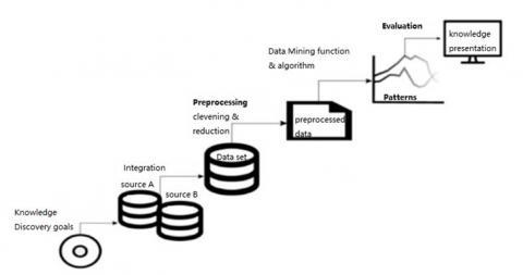
Data mining is the process of extracting, identifying, and analyzing various information to find patterns in data using mathematical techniques, artificial intelligence, statistics, and machine learning. Based on the tasks that can be performed, data mining is grouped into several parts, namely decryption, prediction, estimation, classification, clustering, and association [13]. The term data mining is often referred to as knowledge discovery in database (KDD), the following stages in the data mining process are shown in the Figure 1.
Figure 1. Stages of data mining
In Figure 1, there are several stages of the process of data mining. The first stage is the collection of the dataset that will be used, then continued with the pre-processing stage and the third stage is the data mining process using the existing dataset. Then, the last stage is an evaluation to determine the performance results of the method proposed in this study.
2.1 Data
The diagnosis of TB is carried out by undergoing a bacteriological examination to confirm TB disease. Bacteriological examination refers to the examination of smears from biological preparations (sputum or other specimens), examination of cultures, and identification of Mycobacterium tuberculosis. Currently, the TCM test with Xpert MTB/RIF is the only molecular test that covers all the necessary reaction elements, including all the reagents needed for the PCR (Polymerase Chain Reaction) process.
The features or criteria used for the classification process are explained respectively as follows:
(1) Age, in the form of a numerical feature that contains information about the age of each sample. Based on age group, the older a person is, the higher the risk of developing TB. The older the age, the immune system will also decrease so that it is easy to catch the disease [14].
(2) The sex criterion is a category data feature that contains information on the patient sample's gender. Judging from the analysis, men are also susceptible to TB disease because it is seen from smoking habits that cause TB disease [14].
(3) Chest X-ray, in the form of a category feature that contains information about the results of the chest X-ray test. Positive if TB is found and negative if not found. This is done to ensure the coexistence of pulmonary TB [15].
(4) HIV status, in the form of a category feature that contains information about the HIV status of each patient. Positive if you have HIV and negative if you don't. Tuberculosis in HIV/AIDS (TB-HIV) patients is often found with a prevalence of 29-37 times more than TB without HIV [8].
(5) Diabetes history, in the form of a category feature that contains information about the sample patient's history of diabetes. Diabetes is one of the most common risk factors in pulmonary TB patients. Currently, the prevalence of pulmonary TB is increasing along with the increasing prevalence of diabetes patients. The frequency of diabetes in TB patients is reported to be around 10-15% and the prevalence of this infectious disease is 2-5 times higher in diabetic patients compared to non-diabetics [8].
(6) Whereas the TCM result feature is in the form of a category feature that contains information on the results of the TCM test for each individual sample with a value; resistant rif, sensitive rif, and negative. Rif-resistant TB patients are patients who experience resistance to the antibiotic drug rifampicin. Sensitive rif is a test that has confirmed TB but is not resistant to antibiotics. Negative, namely the result that no TB bacteria are found in the lungs.
This research was conducted to be able to classify the types of TB disease based on the anatomical location suffered by individuals by using features in the dataset used to determine the type of TB suffered. Extrapulmonary TB cases are almost always non-infectious, unless the patient also has pulmonary TB because 50-60% of HIV-positive people infected with TB will develop pulmonary TB disease [8]. Meanwhile, to find out if an individual has extrapulmonary TB, it is necessary to carry out a bacteriological test by carrying out a direct microscopic examination, TCM TB [8]. The results of chest x-rays are also needed to be able to classify an individual as a patient with pulmonary TB or extrapulmonary TB.
2.2 Data pre-processing
Data pre-processing starts with data transformation to convert categorical data into numeric so that later the data can be processed. The next process is data imputation to overcome the missing value condition. After the imputation of data, the next step is to normalize the data so that the data used has a value range of 0 to 1.
2.3 Data transformation
Data transformation is a change in the scale of data to other forms so that the data has a distribution as expected. Each data will perform the same mathematical operation on the original data [16]. Changes to all data are intended to keep differences between data relatively constant. If the data exceeds one variable, all variables will be transformed so that the relationship between the data does not change. The data transformation carried out in this study is to change the value in the categorical dataset to be converted to numeric data.
2.4 Imputation missing value
The missing value is a condition where there is value or information on a subject that is missing. The causes of this missing value vary, it can be due to an error in data collection or the data is not readable in the system so the value is considered missing [6]. There are several methods to overcome the missing value condition, one of which is the imputation process using the KNN (K-Nearest Neighbor) method.
KNN is an imputation method that is based on data by finding the shortest distance to the object data [17]. By implementing this method, it aims to determine the value of a new object based on attribute values and training samples besides that because this method classifies based on the closest distance which is implemented in a simple formulation
The closest distance is calculated using the Euclidean formula with the following equation:
$d(a, b)=\sum_{i=1}^n(X i-Y i)^2$ (1)
where,
d(a, b): Euclidean distance
Xi: first data
Yi: second data
i: Attribute i
n: Number of attributes
2.5 Data normalization
Data normalization is a process to change several variables so that they have the same value range, no data is too large or too small so it will be easier to perform statistical analysis. The method used to normalize tuberculosis data is the Min-Max Normalization method [18]. The equation below is a formula for the min-max normalization method.
$z=\frac{x-\min (x)}{[\max (x)-\min (x)]}$ (2)
where,
z: normalization result
x: value x (original)
min(x): the minimum value for the variable x
max(x): the maximum value for the variable x
2.6 Data mining process
In this study, the data mining process involves the process of balancing data and sharing training data and test data. Data balancing is a process to equalize the amount of data in each class to improve the accuracy of the system during the learning process [19]. In this stage, learning the classification model was carried out, namely grouping TB data into pulmonary and extrapulmonary class categories. The number of TB patient data is 985, the extrapulmonary class is 271, while the pulmonary class has a larger number with a total of 714 data. There is no specific size for a dataset that is said to be unbalanced data, but if you look at the data used in this study there are large and very striking differences in the amount of data for each class. So that it can be said for the data used in this study is data with an unbalanced number of classes. On this occasion, the oversampling technique was used to balance the data using the SMOTE (Synthetic Minority Oversampling Technique) method. The way the SMOTE method works is by replicating the data randomly by choosing k closest neighbors as the determinant, then the minority data set will be balanced with the majority data.
From this explanation, it can be formulated into the following formula [20].
dist $=\sqrt{\left(X_1-X_1\right)^2+\left(X_2-X_2\right)^2+\cdots+\left(X_n-X_n\right)^2}$ (3)
$X_{s y n}=X_i+\left(X_{k n n}-X_i\right) \delta$ (4)
where,
Xi=vector of features in the minority class
Xknn=k-nearest neighbors for Xi
$\delta$=random number between 0 to 1
After balancing the data, the next step is to divide the data set into k to n partitions.Splitting this data is known as K-Fold Cross Validation and is a popular method of solving statistical data where the data is divided into two subsets, namely training data for the learning process and test data for validation or assessment used to assess performance models, methods, or algorithms [19]. K-Fold cross validation can be selected based on dataset size. Usually K-Fold is used to reduce computation time and also maintain the accuracy of the estimation. The size of the shared data depends on the specified K value. In this study, a k-fold value of 10 is used. In each iteration, the original dataset provided is divided randomly by cross-validation into training sets, which are used to train the machine learning algorithm, and tests are determined to evaluate its performance [21, 22].
In the data mining process, various methods can be used to build a classification model to be applied to a TB disease diagnosis system, including Naive Bayes, Support Vector Machines, or the application of branches of deep learning methods such as LSTM and Backpropagation.
2.7 Naive Bayes
A technique derived from Bayes' theorem for classifying data is the Naive Bayes Classifier. This method can predict future data based on past data or existing data by calculating odds from test data with data stored in the training process [23, 24]. Its main feature is a very strong (naive) assumption of independence, regardless of any circumstances or events [10]. Bayes theorem is the basis of this method. So, before we get into the explanation of Nave Bayes, let's first explain Bayes' theorem. If there are two separate events in Bayes' theorem (e.g., A and B), then Bayes' theorem can be written using the following formula:
$P(A \mid B)=\frac{P(A)}{P(B)} P(B \mid A)$ (5)
where,
A: Classless data
B: Data hypothesis
P(B|A): Probability of hypothesis B against condition A
P(B): Probability hypothesis B
P(A|B): Probability of A based on condition of B
P(A): Probability A
The application of the law of total probability Bayes theorem can be developed into the following equation:
$P(A \mid B)=\frac{P(A) P(B \mid A)}{\sum_{1-1}^n P(B \mid A)}$ (6)
where, the variables F1 through Fn represent the characteristics of the statements required to complete the classification, while the variable C is a class. Thus, the above formula shows that the probability of including a sample with certain characteristics in class C is equal to the probability of class C occurring (before the sample was included, or what is called a prior) multiplied by the probability of occurrence of the global one Sample characteristics (evidence). Therefore, the equation x above can be formulated using the following equation:
$Posterior=\frac{\text { prior } x \text { likehood }}{\text { evidence }} v$ (7)
The value of evidence is always fixed for each class in one sample. The value of the Posterior will be compared with the Posterior values of other classes to determine to what class a sample will be classified.
2.8 Support vector machine
SVM (Support Vector Machine) is one method for predicting, both regression and classification cases [18]. The basic principle of SVM uses a linear classifier. A linear classifier is a classification case that is separated linearly, but SVM has evolved to work in non-linear cases by using the kernel concept in high-dimensional workspaces. Hyperplanes are used for high-dimensional spaces that aim to maximize the distance (margin) between data classes [25]. The best separator function (hyperplane) must be found among the unlimited number of other hyperplanes in order to find the optimal separator function (classifier) and separate two different classes. The best hyperplane is the one that is right between two sets of objects of two classes.A hyperplane can be said to be the best if it is located right between two sets of objects from two classes. Figure 2 shows how SVM maximizes the distance between two different sets of classes (margins) by determining the best hyperplane.
Figure 2. SVM finds the best hyperplane to separate class-1 from class+1
Figure 2 shows how the hyperplane is used as a separator of two different classes in the classification process to achieve good results, by measuring the hyperplane margin and determining the maximum point. The distance between the hyperplane and the closest pattern of each class is called the margin [26]. In the Figure 2, the dotted line represents the pattern closest to the hyperplane, which is called the support vector. A hyperplane will be used as the largest class separator by the SVM algorithm. The dividing line between the two classes forms an equation:
$\begin{aligned} & x_i \cdot w+b \geq 1 \,\,\,\,\,\,\,\, \text { untuk } y_i=+1 \\ & x_i \cdot w+b \leq 1 \,\,\,\,\,\,\,\, \text { untuk } y_i=-1\end{aligned}$ (8)
From these equations, it can be seen that the data that falls into the first-class category is data that has a larger equation value, while the data that enters the second-class category is data that has a smaller equation value. The value of the margin or the value of the distance between the boundary planes based on the formula for the distance of the line to the center point can be represented by the equation below:
$\frac{1-b-(-1-b)}{\|w\|}=\frac{2}{\|w\|}$ (9)
Then this margin value will be maximized by minimizing the value of $\|w\|$ as the denominator. This can be formulated as Quadratic Programming. If the two boundary planes are represented as Eq. (9), the search for the dividing line with the largest boundary can be formulated as follows:
$y_i \left(x_i \cdot w+b\right)-1 \geq 0$ (10)
$\min \frac{1}{2}\|w\|^2$ (11)
This problem can be solved by existing computational techniques, such as the Lagrange multiplier expressed in Eq. (12).
$L(w, b, a)=\frac{1}{2\|w\|^2}-\sum_{i=1}^l a_i\left(y_i((\vec{x} \vec{w}+. .+\mathrm{b})-1)\right)$ (12)
$\sum_{i=1}^l a_i-\frac{1}{2} \sum_{i, l=1}^l a_i a_j y_i y_j x_i, x_j$ (13)
where,
$a_i \geq 0 (i=1,2, \ldots l) \sum_{i, l=1}^l a_i y_i=0$ (14)
where,
w: weight vector
x: attribute input value
b: bias
ai: support vector
yi: data class
If the data cannot be separated linearly, it can be said that the classes in the input space cannot be separated perfectly. This causes the constraint in Eq. (9) is not met, so the optimization cannot be done. To overcome these problems, SVM is formulated using the soft margin technique, the following is the mathematical equation:
$y_i \left(x_i \cdot w+b\right) \geq 1-\varepsilon_i$ (15)
Thus, Eq. (15) is converted into an equation as below:
$\min _w=\frac{1}{2}\|w\|^2+c \sum_{i=1}^l \varepsilon_i$ (16)
where,
w=weight vector
x=attribute input value
b=bias
$\varepsilon_i$=error value
c=constant value
In general, the problems that exist rarely have linear separable data and most of them are non-linear. Solving the non-linear SVM problem is to map the x data by a function $\phi(x)$ to a vector space with a higher dimension. In the new vector space, a hyperplane that separates the two classes can be constructed. Then do the dot product calculation from the data that has been transformed in a higher dimensional space, namely $\phi\left(x_i\right)$. $\phi\left(x_i\right)$. However, in general, the transformation $\phi$ is difficult to understand, therefore the dot product value search can be replaced with a kernel function as in the following equation:
$K\left(x_i, x_j \phi\left(x_i\right) \cdot \phi\left(x_j\right)\right)$ (17)
The following are kernel functions that are commonly used to classify non-linear data [11]:
1. Linear Kernel
$K\left(x_i, x\right)=x_i^T x$
2. Kernel Polynomial
$K\left(x_i, x\right)=\left(\gamma x_i^T+r\right)^p, \gamma>0$
3. Kernel RBF or Radial Based Function
$\mathrm{K}\left(x_i, x\right)=\exp \left(-\gamma\left\|x-x_i\right\|^2\right)$
4. Sigmoid Kernel
$K\left(x_i, x\right)=\tanh \left(\gamma x_i^T+r\right)$
2.9 Backpropagation
Backpropagation is a supervised learning algorithm that uses multiple layers to change the weights connected to the neurons in the hidden layer [27]. The Backpropagation algorithm minimizes errors in the output generated by the network by changing the value of its weights in the backward direction using the output error. To get the error output, the forward step must be done first. In the Backpropagation algorithm, the training process is carried out in two phases, namely the forward propagation and backward propagation stages [27]. The following is the algorithm flow of backpropagation in each phase.
Phase 1: Forward Propagation
(1) Initialize the weight with a small random value, maximum Epoch value, error value, and learning rate.
(2) Perform the steps below when the epoch value is smaller than the maximum value.
(3) Each input unit receives the signal and forwards it to the hidden unit.
(4) Calculate all outputs on hidden units zk (j=1, 2, …, p).
$z_{-}net_j=v_{j o}+\sum_{i=1}^n x_i+v_i$ (18)
$z_j=f\left(z_{-} n e t_j\right)=\frac{1}{1+e^{-z_{-} n e t}}$ (19)
•Calculate all network outputs in units of yk (k=1, 2, …, m)
$y_{-} n e t_k=w_{k o}+\sum_{j=1}^p z_i+w_{k j}$ (20)
$y_k=f\left(y_{-} n e t_j\right)=\frac{1}{1+e^{-y \_n e t}}$ (21)
Phase 2: Backward Propagation
•Calculate the output unit factor based on the error value for each output unit yk (k=1, 2, ..., m).
$\delta_k=\left(t_k-y_k\right) f^{\prime} Ynet _j=\left(t_k-y_k\right) y_k\left(1-y_k\right)$ (22)
•Calculate the weight correction using the formula below.
$\Delta W_{j k}=\mathrm{a} \delta_k z_y ; k=1,2, \ldots, m ; j=0,1, \ldots p$ (23)
•Calculate the weight correction using the formula below yk (k=1, 2, ..., m).
$\delta_{-} n e t j=\sum_{k=1}^m \delta_k W_{k j}$ (24)
$\delta_j=\delta_{\_} n e t_j f^{\prime} Znet_j=\delta_{n e t j} Z_j\left(1-z_j\right)$ (25)
•Calculate the weight correction using the formula below.
$\Delta V_{j i}=\mathrm{a} \delta_j x_j ; j=1,2, \ldots, m ; i=0,1, \ldots p$ (26)
•Add up the change in weight of the line leading to the output unit.
$\begin{gathered}W_{j k}(\text { new })=W_{j k}(\text { old })+\Delta W_{j k}; \\ k=1,2, \ldots, m ; j=0,1, \ldots p\end{gathered}$ (27)
Add up the change in weight of the line leading to the hidden unit.
$\begin{gathered}\Delta V_{j i}(\text { baru })=V_{j i}(\text { lama })+ \Delta V_{j i} ; \\ \quad j=1,2, \ldots, m ; i=0,1, \ldots p\end{gathered}$ (28)
where,
w0k: bias weight on output unit yk
v0j: bias weight on hidden unit zj
vij: line weight from unit to hidden unit zj
wjk: line weight from zj to output unit yk
fk: activation function on the hidden unit to output
fj: activation function on input unit to hidden
zj: j-th hidden unit
yk: k-th output unit
i: 1…, n
j: 1…, p
k: 1…, l
n: number of input units
p: number of hidden units
l: number of output units
2.10 Long Term Short Memory (LSTM)
Long Term Short Memory (LSTM) is a development of a neural network that is used to model data in a certain time series. This method can also overcome long-term dependence on the input. Cells in the LSTM store a value, either for a long or a short period of time. The memory block in the LSTM determines which value will be selected as the relevant output for the given input [12]. This LSTM method is proposed as a solution to overcome the vanishing gradient problem on the RNN when processing long sequential data.
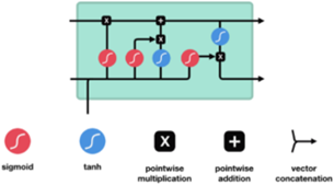
Figure 3 illustrates the architecture of the LSTM. There are four activation function processes at each input to neurons, hereinafter referred to as gate units. The gate units are forgotten gates, input gates, cell gates, and output gates [9]:
Figure 3. LSTM architecture
1. Forgot gates
The input data will be processed and it will be chosen which one will be used or discarded in the memory cells. The sigmoid activation function is used in this gate, which results in a value between 0 and 1 [16]. If the output is 1 then all data will be stored and vice versa if the output is 0 then all data will be discarded. With the following formula [28]:
$f t=\sigma\left(W_f\left[h_{t-1}, x_t\right]+b_f\right)$ (29)
where,
ft: forget gate
$\sigma$: sigmoid activation function
Wf: weights forget gate
xt: input cell
ht-1: output cell previously
bf: bias forget gate
2. Input gates
The 2 gates are in the input state, which must first decide which value to replace using the sigmoid function. Then, the tanh activation function will create a new value vector and store it in the memory cell. With the following formula:
$i_t=\sigma\left(W_i\left[h_{t-1}, x_t\right]+b_i\right)$ (30)
$c_t=\tanh \left(W_c\left[h_{t-1}, x_t\right]+b_c\right)$ (31)
where,
it: input gate
wi: weights input
bi: bias input gate
Ct: candidate
tanh: tanh activation function
Wc: weights candidate
3. Cell gates
The cell gates replace the value in the previous memory cell with the new memory cell value. This value is obtained by combining the values contained in the forget gate and the input gate. With the following formula:
$\left.c_t=f_t * c_{t-1}+i_t * c_t\right)$ (32)
where,
ct: cell state
ct−1: cell state previously
4. Output gates
Two gates must be implemented at the output gates. First, the sigmoid activation function is used to decide which part of the memory cell value to output. Next, the value is inserted into the memory cell using the activation function tanh. Finally, the two gates are multiplied to give the value to be output. With the following formula:
$o_t=\tanh \left(W_o\left[h_{t-1}, x_t\right]+b_o\right)$ (33)
$h_t=o_t * \tanh$ (34)
where,
Ot: output gate
Wo: weights output gate
bo: bias output gate
ht: the hidden layer
2.11 Evaluation
In modeling the classification process, it is necessary to evaluate the performance of the system to measure how well the method used [29]. The method commonly used in evaluating the system is the confusion matrix. A confusion matrix is one method of evaluating the calculation of the level of accuracy, precision results, recall, and f-measure of the algorithm used in research and is measured from the results of testing data that have been predicted [30].
Accuracy is the value of the effectiveness of the overall results of the classification process, following the formula:
(1) Accuracy is the value of the effectiveness of the overall results of the classification process, following the formula:
$Accuracy=\frac{T P+T N}{T P+T N+F P+F N}$ (35)
(2) Precision is the result of the percentage of positive classification data labels, following the formula:
$Precision=\frac{T P}{T P+F P} \times 100 \%$ (36)
(3) The recall is the result of the effectiveness of the classification process for the identification of positive labels, the following formula is:
$Recall=\frac{T N}{T N+F N} \times 100 \%$ (37)
F-measure is the result of mean recall and precision, where the range of f-measure itself is 0-1.
$F-measure=2 \times \frac{\text { Recall } \times \text { Precision }}{\text { Recall }+ \text { Precision }} \times 100 \%$ (38)
where,
TP: the number of data correctly predicted positive.
TN: the number of data with the original class is positive but the prediction result is negative.
FN: the number of data correctly predicted negative.
FP: the number of data with the original class is negative but the prediction result is positive.
3.1 Data collection
The data used in this classification process is Bangkalan residents' tuberculosis data which consists of 985 records and 6 attributes, namely age, gender, chest X-ray, HIV status, history of diabetes, and TCM results. In the data used, there is a missing value which will be overcome by implementing the imputation process using the KNN method [4, 31]. The mission value in the dataset can be seen in Table 1.
Table 1. Number of blank data on each attribute
|
Attribute |
Number of Blank Data |
|
Age |
0 |
|
Sex |
0 |
|
Thorax X-Ray |
28 |
|
HIV |
261 |
|
Diabetes |
7 |
|
TCM |
439 |
3.2 Analysis
Figure 4 describes the IPO diagram as follows:
Figure 4. Process flowchart
(1) Data input process
In this process, the input data used for the classification process is data on patients with TB disease with 6 features.
(2) Data pre-processing
At this stage, the SMOTE process is carried out to balance the data so that the amount of data in each class is balanced. Balancing the data is done by oversampling the minority class, namely the data with the negative class so that the number is balanced with the positive class. The amount of data in the pulmonary class is 596, while the extra lung is 389. So a method is needed to balance the data [19]. This method works by replicating the data randomly by choosing KNN as the determinant, then the minority data set will be balanced with the majority data. The value of k used in this study is k=5.
(3) Data balancing process
At this stage, the SMOTE process is carried out to balance the data so that the amount of data in each class is balanced. Balancing the data is done by oversampling the minority class, namely the data with the negative class so that the number is balanced with the positive class. This method works by replicating the data randomly by choosing k closest neighbors as the determinant, then the minority data set will be balanced with the majority data. The value of k used in this study is k=5.
(4) Data sharing process
The k-fold cross validation method is used to divide training data and test data by k-fold 10. Training data is used in building models with a certain amount of data, while test data is the remaining data that is not used during training to test model performance who have been trained.
(5) Classification process
At this stage, the learning process is carried out to obtain a classification model using several different methods, namely Naïve Bayes, Support Vector Machine, Backpropagation, and LSTM. The different classification models will be compared to the accuracy results to obtain optimal classification results.
(6) Output
After the entire process is run, it will produce an output in the form of class predictions from TB attributes based on modelling with the method proposed in this study.
3.3 Naive Bayes
The results obtained by applying the TB dataset using the Naïve Bayes algorithm combined with KNN for handling incomplete data or missing values, as well as using the SMOTE method and without SMOTE will then be tested using a different number of k cross-validations (k), namely k -fold which amounts to 1 to 10.
Table 2. Evaluation results using the Naive Bayes method in percent
|
Fold |
With SMOTE |
Without SMOTE |
||||||
|
Acct |
Prcs |
Rcl |
F1-S |
Acct |
Prcs |
Rcl |
F1-S |
|
|
1 |
98.9 |
96.4 |
100 |
98.2 |
98.9 |
95.2 |
100 |
97.5 |
|
2 |
100 |
100 |
100 |
100 |
100 |
100 |
100 |
100 |
|
3 |
100 |
100 |
100 |
100 |
98.9 |
97.2 |
100 |
98.6 |
|
4 |
100 |
100 |
100 |
100 |
98.9 |
96.6 |
100 |
98.3 |
|
5 |
98.9 |
97.0 |
100 |
98.5 |
100 |
100 |
100 |
100 |
|
6 |
97.9 |
93.5 |
96.6 |
100 |
100 |
100 |
100 |
100 |
|
7 |
100 |
100 |
100 |
100 |
100 |
100 |
100 |
100 |
|
8 |
98.9 |
99.3 |
98.3 |
98.8 |
100 |
100 |
100 |
100 |
|
9 |
98.9 |
94.7 |
100 |
97.3 |
98.9 |
95.8 |
100 |
97.8 |
|
10 |
100 |
100 |
100 |
100 |
98.9 |
97.1 |
100 |
98.5 |
|
Avg |
99.4 |
98.2 |
100 |
99.1 |
99.4 |
98.2 |
100 |
99.0 |
|
RT |
5.87(s) |
2.80(s) |
||||||
where,
Acct: accurate
Prcs: precission
Rcl: recall
F1-S: F1-Score
Avg: average
RT: running time
Table 2 shows that the average accuracy is 99.4% with a computation time of 5.87 seconds when the SMOTE method is applied, while without SMOTE the average accuracy is also 99.4% with a computation time of 2.08 seconds.
The advantages of Naive Bayes can be used for both quantitative and qualitative data. No need to do a lot of data training. If there is a missing value, it can be ignored in the calculation, and the calculations are fast and efficient so that they are easy to understand. While the weakness of naive Bayes is assuming that each variable is independent so that it reduces accuracy because usually there is a correlation between one variable and another.
3.4 Support vector machine
At this stage, the research is carried out by making trial scenarios to draw the right conclusions after the research process is carried out. The trial scenarios carried out in this study are described in Table 3:
Table 3. Testing scenarios
|
No. |
Trial Scenario |
Parameter |
|
1 |
K-Fold Value |
K= 1 to K=10 |
|
2 |
Kinds of Kernel |
Linear, Polynomial, RBF, Sigmoid |
|
3 |
C value |
0,5; 1; 10; 100 |
|
4 |
Gamma Scales |
Scale; 1; 0,1; 0,01; 0,001; 0,0001 |
Based on the parameters in the test scenario, the best parameters are then searched for by optimizing the parameters using Grid Search. The use of grid search in the pilot scenario for parameter optimization is intended so that the parameter optimization process does not take much time. The results of the experiments were carried out using the best parameters from the results of parameter tuning using the Grid Search method. The best parameters obtained from the SVM model as shown in Table 4.
Table 4. Best parameters of gird search results
|
Kernel Coefficient (gamma) |
Scale1 / $\left(n_{-}\right.$features $*$ $X . \operatorname{var}())$ |
|
Regulation Value (C) |
0.5 |
|
Kernel |
RBF (Radial Basis Function) |
From the best parameters obtained, it will be applied to the classification process with the SMOTE method and without SMOTE and then will be tested using a different number of k cross-validations (k), namely k-fold which amounts to 1 to 10. The test results can be seen in Table 5.
Table 5. Evaluation results using SVM in percent
|
Fold |
With SMOTE |
Without SMOTE |
||||||
|
Acct |
Prcs |
Rcl |
F1-S |
Acct |
Prcs |
Rcl |
F1-S |
|
|
1 |
98.6 |
98.7 |
98.5 |
98.6 |
98.9 |
99.3 |
98.0 |
98.6 |
|
2 |
100 |
100 |
100 |
100 |
98.9 |
99.3 |
98.0 |
98.6 |
|
3 |
98.3 |
99.3 |
99.3 |
99.3 |
98.9 |
99.3 |
98.0 |
98.6 |
|
4 |
98.6 |
98.4 |
98.7 |
98.6 |
97.9 |
98.6 |
96.6 |
97.5 |
|
5 |
99.3 |
99.3 |
99.3 |
99.3 |
100 |
100 |
100 |
100 |
|
6 |
99.3 |
99.4 |
99.2 |
99.3 |
100 |
100 |
100 |
100 |
|
7 |
100 |
100 |
100 |
100 |
98.9 |
99.3 |
98.1 |
98.7 |
|
8 |
100 |
100 |
100 |
100 |
100 |
100 |
100 |
100 |
|
9 |
100 |
100 |
100 |
100 |
100 |
100 |
100 |
100 |
|
10 |
98.5 |
98.7 |
98.5 |
98.6 |
100 |
100 |
100 |
100 |
|
Avg |
99.3 |
99.3 |
99.3 |
99.3 |
99.3 |
99.5 |
98.8 |
99.2 |
|
RT |
0.18(s) |
0.08(s) |
||||||
Table 5 shows that the average accuracy is 99.3% with a computing time of 0.18 seconds when the SMOTE method is applied, while without SMOTE the average accuracy is 99.3% with a computation time of 0.08 seconds.
When the data are not linearly separated, the kernel RBF is a kernel function that is frequently employed in analysis. Gamma and Cost are the two parameters that make up the RBF kernel. Parameter The parameter cost, often known as C, is used as an SVM optimization to prevent misclassification in each sample in the training dataset. A low value for the Gamma parameter indicates "far" influence while a high value indicates "close" influence of a sample training dataset. Low gamma makes it reasonable to take into account locations that are far from the separator line while determining the separator line. When the gamma is large, the points should be taken into account in the computations because they are near the line.
The benefit of the SVM method is that it can function reasonably well when there is a distinct line of demarcation between classes, saves more memory because it uses training points from the decision function (support vector), and is effective when the number of dimensions is greater than the number of samples. This method's difficulty in using it to sets with a lot of dimensions is its flaw.
3.5 Backpropagation
The use of the Backpropagation method is done by making a test scenario to draw the right conclusions after the research process is carried out. The trial scenarios carried out in this study are described in Table 6.
Table 6. Testing scenarios on the backpropagation method
|
No. |
Trial Scenario |
Parameter |
|
1 |
Fold |
K=1 to K=10 |
|
2 |
Number of Neurons |
60-100 |
|
3 |
Optimization |
Adam Optimizer |
|
4 |
Activation Functions |
Sigmoid |
|
5 |
Learning Rate |
0.001 |
|
6 |
Epoch |
25 |
The test uses the sigmoid activation function with the number of neurons being 60 and without using optimization. Experiments using k-fold 10 and a learning rate of 0.001 with many iterations (epochs) of 25. The Table 7 is the result of tests carried out on data with SMOTE and without SMOTE.
Table 7. Test results using backpropagation with Epoch=25 percent
|
Fold |
With SMOTE |
Without SMOTE |
||||||
|
Acct |
Prcs |
Rcl |
F1-S |
Acct |
Prcs |
Rcl |
F1-S |
|
|
1 |
100 |
100 |
100 |
100 |
100 |
100 |
100 |
100 |
|
2 |
100 |
100 |
100 |
100 |
100 |
100 |
100 |
100 |
|
3 |
100 |
100 |
100 |
100 |
98.9 |
99.3 |
98.0 |
98.6 |
|
4 |
100 |
100 |
100 |
100 |
100 |
100 |
100 |
100 |
|
5 |
99.3 |
99.2 |
99.3 |
99.3 |
100 |
100 |
100 |
100 |
|
6 |
100 |
100 |
100 |
100 |
98.9 |
99.3 |
97.8 |
99.8 |
|
7 |
100 |
100 |
100 |
100 |
100 |
100 |
100 |
100 |
|
8 |
99.3 |
99.3 |
99.3 |
99.3 |
99.3 |
99.3 |
99.3 |
99.3 |
|
9 |
100 |
100 |
100 |
100 |
100 |
100 |
100 |
100 |
|
10 |
99.2 |
99.4 |
99.2 |
99.2 |
98.9 |
99.3 |
99.3 |
98.7 |
|
Avg |
99.7 |
99.7 |
99.7 |
99.7 |
99.7 |
99.7 |
99.4 |
99.6 |
|
RT |
38.61(s) |
31,75 (s) |
||||||
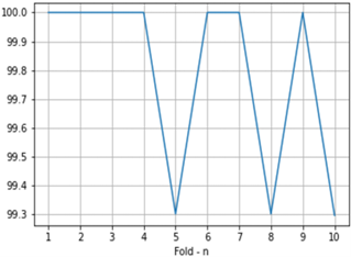
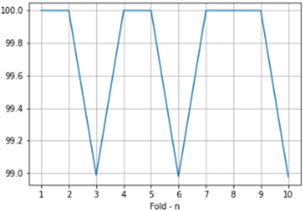
Figures 5 and 6 show that the average accuracy is 99.7% with a computation time of 38.61 seconds when the SMOTE method is applied, while without SMOTE the average accuracy is also 99.6% with a computation time of 31.75 seconds. The most prominent advantages of the Backpropagation algorithm are Fast, simple, and easy to program. Has no tuning parameters other than the number of inputs. Flexible because it does not require prior knowledge of the network. while the weakness of Backpropagation is that it takes a long time in the learning process.
Figure 5. Accuracy results at Epoch=25 with SMOTE
Figure 6. Accuracy results at Epoch=25 without SMOTE
3.6 LSTM
The use of the LSTM method is carried out by making a test scenario to draw the right conclusions after the research process is carried out. In this study, two kinds of tests were carried out, namely, the parameter values to be used and testing for the removal of features that had the greatest missing value to see the effect of the accuracy results obtained. The test scenario for the parameters used is described in Table 8 and the test for the effect of the feature that has the largest number of missing values can be seen in Table 9.
Table 8. LSTM testing scenarios
|
No. |
Trial Scenario |
Parameter |
|
1 |
Fold |
K=1 to K=10 |
|
2 |
Number of Neurons |
60-100 |
|
3 |
Optimization |
Adam Optimizer, SGD, |
|
4 |
Activation Functions |
Sigmoid, Tanh |
|
5 |
Learning Rate |
0.01, 0.001 |
|
6 |
Epoch |
25 |
Table 9. Best parameters of gird search results
|
Number of Neurons |
100 |
|
Optimization |
Adam Optimizer |
|
Activation Functions |
Tanh |
|
Learning Rate |
0.01 |
Table 10. Test results using LSTM with 100 neurons and Epoch=25 percent
|
Fold |
With SMOTE |
Without SMOTE |
||||||
|
Acct |
Prcs |
Rcl |
F1-S |
Acct |
Prcs |
Rcl |
F1-S |
|
|
1 |
100 |
100 |
100 |
100 |
100 |
100 |
100 |
100 |
|
2 |
100 |
100 |
100 |
100 |
100 |
100 |
100 |
100 |
|
3 |
100 |
100 |
100 |
100 |
100 |
100 |
100 |
100 |
|
4 |
100 |
100 |
100 |
100 |
100 |
100 |
100 |
100 |
|
5 |
100 |
100 |
100 |
100 |
100 |
100 |
100 |
100 |
|
6 |
100 |
100 |
100 |
100 |
100 |
100 |
100 |
100 |
|
7 |
100 |
100 |
100 |
100 |
100 |
100 |
100 |
100 |
|
8 |
100 |
100 |
100 |
100 |
100 |
100 |
100 |
100 |
|
9 |
100 |
100 |
100 |
100 |
100 |
100 |
100 |
100 |
|
10 |
100 |
100 |
100 |
100 |
100 |
100 |
100 |
100 |
|
Avg |
100 |
100 |
100 |
100 |
100 |
100 |
100 |
100 |
|
RT |
109.08 (s) |
104.90(s) |
||||||
Based on the parameters in the test scenario, the best parameters are then searched for by optimizing the parameters using Grid Search. The test uses the Tanh activation function with the number of neurons being 100 and using the Adam optimizer. Experiments using k-fold 10 and a learning rate of 0.001 with many iterations (epochs) of 25. The Table 10 is the results of tests carried out on data with SMOTE and without SMOTE.
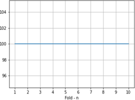
Figures 7 and 8 show that the average accuracy is 100% with a computation time of 109.08 seconds when the SMOTE method is applied, while without SMOTE the average accuracy is also 100% with a computation time of 104.9 seconds.
LSTM helps in the classification process unlike ordinary neural network processes which are all based on activation and weights, the LSTM cell state plays an important role in providing relevant classification results.
Figure 7. Accuracy results at Epoch=25 with SMOTE
Figure 8. Accuracy results at Epoch=25 without SMOTE
Our research results yield several critical conclusions. Firstly, the proposed model in this study effectively addresses the problem of missing values in TB data at Syarifah Ambami Rato Ebu Bangkalan Hospital, utilizing the K-NN method. This approach significantly enhances the integrity and accuracy of the dataset.
Secondly, the application of the Synthetic Minority Over-sampling Technique (SMOTE) has been demonstrated to improve the performance of the model, albeit without a significant increase in accuracy compared to the application of datasets without SMOTE. This finding is particularly evident when considering the computation time required. The use of SMOTE demands more time due to the generation of synthetic data to counterbalance the minority data class.
Thirdly, it is concluded that Long Short-Term Memory (LSTM) is highly efficacious in classifying TB disease. Utilizing the GridSearch method, the best accuracy results manifest in several test scenarios, yielding a stable accuracy value of 100% in experiments using 10-fold cross-validation, a learning rate of, and the application of the Tanh activation function on 100 neurons, irrespective of the use of SMOTE.
Fourthly, a comparison of the LSTM method with other methods, such as Naive Bayes, SVM, and backpropagation, establishes the superiority of LSTM in terms of accuracy. LSTM achieves a perfect score of 100%, compared to Naive Bayes (99.4%), SVM (99.3%), and backpropagation (99.7%).
Lastly, our research successfully models a classification of TB disease based on anatomical locations, namely the lungs and extrapulmonary sites, using the LSTM method, thereby enhancing the performance of the algorithm to achieve optimal accuracy. This study contributes to research development by formulating a classification model that can be applied to TB data and offer valuable recommendations to hospitals regarding pulmonary and extrapulmonary classes and significant features of TB disease.
Based on these conclusions, several recommendations emerge for future research. As the next step in system development, it would be beneficial to construct a classification model utilizing another imputation method capable of combining two different types of data. This approach could potentially offer more nuanced and accurate classifications.
Moreover, subsequent research should consider expanding the volume of data and features used to build the classification model. This expansion could enhance the performance of the model, granted that the number of missing values and class balance in the utilized dataset is adequately considered.
This research would like to thank the support of Airlangga University and the University of Trunojoyo Madura.
[1] Saputra, R.A., Noviyani, A., Nopsopon, T. Pongpirul, K. (2021). Variation of tuberculosis prevalence across diagnostic approaches and geographical areas of Indonesia. PLOS ONE, 16(10): e0258809. https://doi.org/10.1371/journal.pone.0258809
[2] Gill, C.M., Dolan, L., Piggot, L.M. McLaughlin, A.M. (2021). New developments in tuberculosis diagnosis and treatment. Breathe, 8(1): 210149. https://doi.org/10.1183/20734735.0149-2021
[3] Nasution, M.KM., Elveny, M., Hardi, S. M., Jaya, I., Siregar, M.A. (2020). Identification of tuberculosis (TB) disease based on lung x-rays using extreme learning machine. Journal of Physics: Conference Series, 1566(1): 012085. https://doi.org/10.1088/1742-6596/1566/1/012085
[4] Rochman, E.M.S., Suprajitno, H. (2022). Overcoming missing values using imputation methods in the classification of tuberculosis. Communications in Mathematical Biology and Neuroscience, 2022: 66. https://doi.org/10.28919/cmbn/7538
[5] Emmanuel, T., Maupong, T., Mpoeleng, D., Semong, T., Mphago, B., Tabona, O. (2021). A survey on missing data in machine learning. Journal of Big Data, 8(1): 140. https://doi.org/10.1186/s40537-021-00516-9
[6] Kang, H. (2013). The prevention and handling of the missing data. Korean Journal of Anesthesiology, 64(5): 402-406. https://doi.org/10.4097/kjae.2013.64.5.402
[7] Aini, N., Ramadiani, R., Hatta, H.R. (2017). Sistem pakar pendiagnosa penyakit tuberkulosis. Jurnal Informatika Mulawarman, 12(1): 56-62. http://dx.doi.org/10.30872/jim.v12i1.224
[8] Khan, M.T., Kaushik, A.C., Ji, L., Malik, S.I., Ali, S., Wei, D.Q. (2019). Artificial neural networks for prediction of tuberculosis disease. Frontiers in Microbiology, 10: 395. https://doi.org/10.3389/fmicb.2019.00395
[9] Venkataramana, L., Prasad, D.V.V., Saraswathi, S., Mithumary, C.M., Karthikeyan, R., Monika, N. (2022). Classification of COVID-19 from tuberculosis and pneumonia using deep learning techniques. Medical & Biological Engineering & Computing, 60(9): 2681-2691. https://doi.org/10.1007/s11517-022-02632-x
[10] Berrar, D. (2018). Bayes’ theorem and naive Bayes classifier. Encyclopedia of Bioinformatics and Computational Biology: ABC of Bioinformatics, 403: 412. https://doi.org/10.1016/B978-0-12-809633-8.20473-1
[11] Liu, Z., Xu, H. (2014). Kernel parameter selection for support vector machine classification. Journal of Algorithms & Computational Technology, 8(2): 163-177. https://doi.org/10.1260/1748-3018.8.2.1
[12] Lees, T., Reece, S., Kratzert, F., et al. (2022). Hydrological concept formation inside long short-term memory (LSTM) networks. Hydrology and Earth System Sciences, 26(12): 3079-3101. http://dx.doi.org/10.5194/hess-26-3079-2022
[13] Beniwal, S., Arora, J. (2012). Classification and feature selection techniques in data mining. International Journal of Engineering Research & Technology, 1(6): 1-6.
[14] Marçôa, R., Ribeiro, A.I., Zão, I., Duarte, R. (2018). Tuberculosis and gender-factors influencing the risk of tuberculosis among men and women by age group. Pulmonology, 24(3): 199-202. https://doi.org/10.1016/j.pulmoe.2018.03.004
[15] Majdawati, A. (2010). Uji diagnostik gambaran lesi foto thorax pada penderita dengan klinis tuberkulosis paru. Mutiara Medika: Jurnal Kedokteran dan Kesehatan, 10(2): 180-188. https://doi.org/10.18196/mmjkk.v10i2.1582
[16] Lee, D.K. (2020). Data transformation: A focus on the interpretation. Korean Journal of Anesthesiology, 73(6): 503-508. https://doi.org/10.4097/kja.20137
[17] Anggoro, D.A., Aziz, N.C. (2021). Implementation of K-nearest neighbors algorithm for predicting heart disease using python flask. Iraqi Journal of Science, 62(9): 3196-3219. https://doi.org/10.24996/ijs.2021.62.9.33
[18] Gheorghe, M., Petre, R. The importance of normalization methods for mining medical data. International Journal of Computers & Technology, 14(8): 6014-6020.
[19] Fithriasari, K., Hariastuti, I., Wening, K.S. (2020). Handling imbalance data in classification model with nominal predictors. International Journal of Computing Science and Applied Mathematics, 6(1): 33-37. http://dx.doi.org/10.12962/j24775401.v6i1.6643
[20] Sain, H., Purnami, S.W. (2015). Combine sampling support vector machine for imbalanced data classification. Procedia Computer Science, 72: 59-66. https://doi.org/10.1016/j.procs.2015.12.105
[21] Normawati, D., Ismi, D.P. (2019). K-fold cross validation for selection of cardiovascular disease diagnosis features by applying rule-based datamining. Signal and Image Processing Letters, 1(2): 62-72. http://dx.doi.org/10.31763/simple.v1i2.3
[22] Nti, I.K., Nyarko-Boateng, O., Aning, J. (2021). Performance of machine learning algorithms with different K values in K-fold cross-validation. International Journal of Information Technology and Computer Science, 6: 61-71. https://doi.org/10.5815/ijitcs.2021.06.05
[23] Peling, I.B.A., Arnawan, I.N., Arthawan, I.P.A., Janardana, I.G.N. (2017). Implementation of data mining to predict period of students study using Naive Bayes algorithm. International Journal of Engineering and Emerging Technology, 2(1): 53-57.
[24] Harahap, F., Harahap, A.Y.N., Ekadiansyah, E., Sari, R. N., Adawiyah, R., Harahap, C.B. (2018). Implementation of Naïve Bayes classification method for predicting purchase. In 2018 6th International Conference on Cyber and IT Service Management (CITSM), Parapat, Indonesia, pp. 1-5. http://dx.doi.org/10.1109/CITSM.2018.8674324
[25] Rodríguez-Pérez, R., Bajorath, J. (2022). Evolution of support vector machine and regression modeling in chemoinformatics and drug discovery. Journal of Computer-Aided Molecular Design, 36: 355-362. https://doi.org/10.1007/s10822-022-00442-9
[26] Cristianini, N., Shawe-Taylor, J. (2000). An introduction to support vector machines and other kernel-based learning methods. Cambridge University Press. https://doi.org/10.1017/CBO9780511801389
[27] Simamora, W.S., Lubis, R.S., Zamzami, E.M. (2020). A classification: Using back propagation neural network algorithm to identify cataract disease. Journal of Physics: Conference Series, 1566(1): 012037. https://doi.org/10.1088/1742-6596/1566/1/012037
[28] Sundararajan, G., Sivakumar, P. (2022). LSTM recurrent neural network-based frequency control enhancement of the power system with electric vehicles and demand management. International Transactions on Electrical Energy Systems, 2022: 1281248. https://doi.org/10.1155/2022/1281248
[29] Mehdiyev, N., Enke, D., Fettke, P., Loos, P. (2016). Evaluating forecasting methods by considering different accuracy measures. Procedia Computer Science, 95: 264-271. https://doi.org/10.1016/j.procs.2016.09.332
[30] Chen, R.C., Dewi, C., Huang, S.W., Caraka, R.E. (2020). Selecting critical features for data classification based on machine learning methods. Journal of Big Data, 7(1): 52. https://doi.org/10.1186/s40537-020-00327-4
[31] Rochman, E.M.S., Suprajitno, H. (2022). Comparison of clustering in tuberculosis using fuzzy C-means and K-means methods. Communications in Mathematical Biology and Neuroscience, 2022: 41. https://doi.org/10.28919/cmbn/7335