Maha Raad Hassan*![]() | Shibly Ahmed Al-Samarraie
| Shibly Ahmed Al-Samarraie![]()
© 2023 IIETA. This article is published by IIETA and is licensed under the CC BY 4.0 license (http://creativecommons.org/licenses/by/4.0/).
OPEN ACCESS
Efficient control of air-handling units (AHUs) in heating, ventilating, and air-conditioning (HVAC) systems is crucial for maintaining comfortable conditions while minimizing energy consumption. This study focuses on a multi-input multi-output (MIMO) control design for a nonlinear dynamic model of an AHU in a single thermal zone featuring variable air volume (VAV) properties in cooling mode. The goal is to develop decoupling controllers for the AHU by manipulating the airflow rate and cold water flow rate. An integral sliding mode control based on barrier function is proposed for regulating the humidity ratio of the thermal zone according to the desired characteristics. Subsequently, an integral sliding mode control based on barrier function is combined with an optimal feedback controller using a linear quadratic regulator (LQR) to manage indoor temperature. Additionally, an approximate classical sliding mode differentiator (ACSMD) is designed to estimate unmeasurable states that are used to construct the sliding variable of the second controller. The performance of the proposed control is evaluated through numerical simulations. Results demonstrate the ability of the controllers to guide the humidity and temperature of the thermal zone toward the required values without prior knowledge of the upper bounds on parameter variation, reducing chattering and yielding an optimal robust integral sliding mode control/LQR controller.
HVAC systems, integral sliding mode control, barrier function, MIMO systems, optimal feedback control
Designing of each HVAC system’s control is to provide a suitable and desirable environment for human life and achieve comfortable and justifiable indoor air quality (IAQ). Main part of HVAC is Air-handling units AHU. AHU which provides a desired supply air with specific temperature and humidity. This units constituting of various equipment and mechanical parts. Therefore, the possibility of complete identification and derivation of equations and designing an effective control system by classical methods is impossible and unattainable and it is difficult to obtain an accurate mathematical dynamic model of AHU [1].
The dynamic mathematical model for AHUs is essential to present an effective control method which can operate in an acceptable way taking into account all practical constraints, it is possible to have an overview of the different modelling techniques to best improve the control strategy of the HVAC systems developed in studies [2-4]. Temperature and humidity are the most important controlled parameters (state variables) in air handling units. Humidity is a significant factor affecting both thermal comfort and indoor air quality. Energy efficiency is a major challenge in buildings for maintaining comfortable conditions. Reducing energy losses and improving the dynamic behavior of the system like comfort conditions for temperature and humidity are the primary objectives of HVAC control systems. In order to achieve these objectives, numerous control approaches have been used, such as the decoupling method, which aims to overcome the problem of humidity coupling by eliminating the temperature disturbance completely and not focusing on reducing the recovery time of humidity [5]. A neural fuzzy structure of decoupled parameter self-tuning fuzzy neural PID controller was proposed in the study [6]. Adaptive and learning-based approaches have also been introduced in the study [7]. Seong et al. [8] the authors performed studies of optimal HVAC control methods using Genetic Algorithms that were implemented to both a variable air volume (VAV) air-conditioning system and chilled water system for optimization of the control variables in each system. Robust control system is crucial due to the dynamic uncertainties and external disturbance. Sliding mode control (SMC) is known to be an appropriate strategy for its robustness against external disturbances and little sensitivity to parameter variations under matching conditions. The SMC needs a suitable control law that is a trajectory moves toward the sliding surface and reaches in a finite time and stays on. SMC is introduced [9, 10] which compared the performance of the system with proposed controller versus performance with PID controller to demonstrate the benefit of using SMC to enhance the desired tracking. Two strategies are implemented on nonlinear model nonlinear decoupled sliding mode control and Linear optimal robust H¥ technique, the result showed that the nonlinear decoupled sliding mode control has given better performance [11].
The fuzzy algorithm is used to investigate the stability of a sliding control system by adjusting the parameters in the approach rate, reducing the switching frequency, and weakening chatter [12]. In the study [13], adaptive sliding mode control to overcome the overvalued of controller gain in sliding mode control is proposed. In spite of the specifications of sliding mode controller it has many drawbacks like the chattering effectiveness, the reaching phase, and sensitiveness to matchless uncertainties [14, 15]. Integral sliding mode (ISMC) is one of the SMC strategies that have been proposed to solve these problems, which is looking to remove the reaching phase by enforcing sliding mode during the entire system response [16]. Integral sliding mode based on barrier function is proposed [17] was applied for a DC servo actuator system containing friction, which is enabled the controller to compensate the external disturbance and uncertainty from the first instant. The ISMC is also proposed [18] for unmatched disturbance. Finally, for the purpose of designing an optimal control the LQR was proposed to provide optimally controlled feedback gains to enable the high performance [19].
The structure of this article is as follows: Section 2 introduces the problem statement, while Section 3 describes the system and the dynamic model of the AHU system. Section 4 illustrates the sliding mode controller, and Section 5 presents the proposed control design. The simulation results are demonstrated in Section 6, and Section 7 concludes the paper.
The non-linear model of AHU has MIMO, complex coupling between control variable, time-varying and control input constraints. However, considering humidity as a control target as well as temperature would greatly increase the challenge of developing appropriate control method since coupling of heat and mass transfer is high, leading to two highly coupled control loops for controlling temperature and humidity respectively especially in presence of variation of parameters and external disturbance [20].
This paper suggests designing the two controllers separately. Integral sliding mode based on barrier function is used for controlling humidity ratio. Integral sliding mode based on barrier function coupled with optimal feedback controller using LQR will be used for the second controller to control the indoor temperature. In order to compute the sliding variable of the second control, the time derivative of an error state that computed the difference between the indoor temperature and the desired temperature is needed. But due to the uncertainty in the AHU model, the time derivative of the error function is obtained here via the ACSMD. Proposing ISMC based on barrier function can overcome the problem of needing the prior information of the upper bound of variation of the system parameters and can eliminate chattering phenomena because barrier function is continuous function.
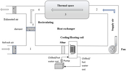
Air handling unit (AHU) is a device used for the control of the air flow quality in HVAC systems. Figure 1 which presents a schematic view of an air-handling unit having one zone (indoor) in HVAC. HVAC system for single thermal load consist of a heat exchanger, a chiller, which provides chilled water to the heat exchanger; a circulating air fan; the thermal space; connecting ductwork; dampers; and mixing air components [9]. A mixed air of 25% of fresh air with 75% of recirculating air passes through the heat exchanger. The temperature and humidity ratio of the hot and humid air are reduced as it passes through the heat exchanger. Finally, the desired supply air is supplied and delivered to the thermal space through the connecting ductwork.
Many assumptions must be considered [9]: 1) Ideal gas behavior; 2) Mixing air should be perfect; 3) Fixed pressure process; 4) Wall and thermal storage must be neglected; 5) thermal losses between components should be negligible; 6) Infiltration and exfiltration effects is neglected; and 7) negligible transient effects in the flow splitter and mixer.
Figure 1. AHU diagram in HVAC systems
The dynamic modeling of the AHU is given in studies [9, 11, 21], by the following differential equations.
$\dot{W}_{i a}=\frac{\dot{M}_l}{\rho_{a d} V_{i a}}-\frac{\dot{f}_{a r}}{V_{i a}}\left(W_{i a}-W_{s a}\right)$
$\dot{T}_{\mathrm{ia}}=\frac{1}{\rho_{a d} C_a V_{i a}}\left(\dot{H}_l-h_v \dot{M}_l\right)+\frac{h_v \dot{f}_{a r}}{C_a V_{i a}}\left(W_{i a}-W_{\mathrm{sa}}\right)-\frac{\dot{f}_{a r}}{V_{i a}}\left(T_{\mathrm{ia}}-T_{\mathrm{sa}}\right)$
$\dot{T}_{s a}=\frac{\dot{f}_{a r}}{V_{c u}}\left(T_{i a}-T_{s a}\right)+\frac{0.25 \dot{f}_{a r}}{V_{c u}}\left(T_{o a}-T_{i a}\right)- \frac{\dot{f}_{a r} h_s}{C_a V_{c u}}\left(0.25 W_{o a}+0.75 W_{i a}-W_{s a}\right)-\frac{\rho_{w d} C_w \delta T_{c u}}{\rho_{a d} C_a V_{c u}} \dot{f}_{w r}$ (1)
The parameters, variables, state and control are described in Tables 1 and 2 [22].
Table 1. Thermo-fluid parameters of AHU
|
Parameters |
|||
|
Via |
Thermmeal space volume |
Woa |
Humidity ratio of outdoor fresh air |
|
Vcu |
Cooling unit volume |
Wsa |
Humidity proportion of Supply air |
|
ρwd |
Water mass density |
Wia |
Thermal zone humidity ratio |
|
ρad |
Air mass density |
Toa |
Outdoor fresh air temperature |
|
hv |
Enthalpy of vapors |
Tsa |
Conditioned air supply temperature |
|
hs |
Enthalpy of saturated water |
Tia |
Thermal zone air temperature |
|
Cw |
Specific heat of water |
δTcu |
Cooling unit temperature gradient |
|
Ca |
Specific heat of air |
$\dot{M}_l$ |
Humidity source strength |
|
$\dot{f}_{a r}$ |
Air flow rate |
$\dot{H}_l$ |
Heat load |
|
$\dot{f}_{w r}$ |
Water flow rate |
|
|
Table 2. Thermo-fluid parameters values in AHU around an operating point
|
Operating point |
|
|
Via=1655.11m3 |
Woa=0.018 kg H2O /kg dry air |
|
Vcu=1.7198m3 |
Wsa=0.007kg H2O/kg dry air |
|
ρwd=1000kg/m3 |
Wia=0.00924kg H2O/kg dry air |
|
ρad=1.185kg/m3 |
Toa=32℃ |
|
hv=2500.45kJ/kg |
Tsa=17℃ |
|
hs=790.84kJ/kg |
Tia=21℃ |
|
Cw=4.183kJ/kg ℃ |
δTcu=6℃ |
|
Ca=1.004kJ/kg ℃ |
$\dot{M}_l=0.021 \mathrm{~kg} / \mathrm{s}$ |
|
$\dot{f}_{a r}=8.02 \mathrm{~m}^3 / \mathrm{s}$ |
$\dot{H}_l=84.93 \mathrm{~kg} / \mathrm{s}$ |
|
$\dot{f}_{w r}=0.00366 \mathrm{~m}^3 / \mathrm{s}$ |
|
In state space form the nonlinear AHU model is given by;
$\begin{aligned} & \dot{x}_1=f_1+g_1 u_1 \\ & \dot{x}_2=f_2 \\ & \dot{x}_3=f_3-g_2 u_2\end{aligned}$ (2)
where,
$f_1=a_1, g_1=-a_2 x_1+a_3$,
$f_2=\left(b_2 x_1-a_2 x_2+a_2 x_3-b_3\right) u_1+b_1$
$f_3=\left(-0.75 c_2 x_1+0.75 c_1 x_2-c_1 x_3+c_3\right) u_1, \quad g_2=c_4$
$u_1=\dot{f}_{a r}, u_2=\dot{f}_{w r}, y_1=W_{i a}, y_2=T_{i a}$
$x_1=W_{i a}, x_2=T_{i a}, x_3=T_{s a}$
$a_1=\frac{1}{\rho_{a d} V i a} \dot{M}_l, a_2=\frac{1}{V_{i a}}, a_3=a_2 W_{s a}$
$b_1=\frac{1}{\rho_{a d} C_a V_{i a}}\left(\dot{H}_l-h_v \dot{M}_l\right), b_2=\frac{h_v}{C_a V_{i a}}$,
$b_3=b_2 * W_{s a}, c_1=\frac{1}{V_{c u}}, c_2=\frac{h_s}{C_a V_{c u}}$,
$c_3=0.25 c_1 T_{o a}-0.25 c_2 W_{o a}+c_2 W_{s a}, c_4=\frac{\rho_{w d} C_w \delta T}{\rho_{a d} C_a V_{c u}}$
Remark (1): According to the physical characteristics for the HVAC system which is represented in Eq. (2), the control inputs are positive quantities. So, the system is non-affine.
SMC has been broadly used to different complicated dynamical systems. SMC consists of two phases reaching phase and sliding phase. The state of the system is derived to the sliding manifold (reaching phase) by applying reaching control law. While in sliding phase, the main appeal of SMC is that it has the capability to compensate matched uncertainties by applying equivalent control and force the state along the sliding surface to the origin [23], as is shown in the study [24]. However, in reaching phase, the systems are sensitive to uncertainties and disturbance. Also designing SMC requires the prior information of the upper bound of variation of parameters and disturbances which is complicated to obtain in practice which is shown in the study [25]. Only overestimation of controller gain can solve this problem and that causes chattering phenomenon which is a serious problem for utilization of sliding modes in control systems. As a solution to this problem, an integral sliding mode control (ISMC) based on barrier function was proposed [17, 26].
4.1 Integral sliding mode
The main idea of ISMC focuses on robustness throughout an entire response. Therefore, Integral Sliding Mode attempts to eliminate the reaching phase. The order of the motion equation in this type of Sliding Mode is equal to the order of the system. Therefore, it is known as the full order sliding mode. As a result, from the first moment instance the robustness of the system can be assured during an entire response of the system [27]. In the ISMC approaches, knowledge of parameters uncertainties bounds is required for the purpose of calculating the control gain, so to overcome this requirement the use of the barrier function is proposed in the present work.
4.2 The barrier function
Instead of discontinuous term of the controller, the barrier function was proposed here which can be defined as:
Definition: Let suppose that $\epsilon$ is a known and constant where ϵ>0, the BF can be defined as an even continuous function $f: x \in[\epsilon, -\epsilon] \rightarrow h(x) \in[\mathrm{g}, \infty]$ strictly increasing on [0, $\epsilon$] [28].
• $\lim _{|x| \rightarrow \epsilon} h(x)=+\infty$.
• h(x) has a unique minimum at zero and h(0)≥0.
There are two different types of BFs are considered;
• Positive definite BFs (PBFs) $: h_p(x)=\frac{\epsilon g}{\epsilon-|x|}$ where h(0)=g> 0.
• Positive Semi-definite BFs (PSBFs): $h_{p s}(x)=\frac{|x|}{\epsilon-|x|}$, where h(0)=0.
4.3 Linear quadratic regulator (LQR)
The LQR is an optimal control algorithm where the principal purpose of optimal control is to determine control signals that will cause a process to satisfy some physical constraints and at the same time (maximize or minimize) a chosen performance index or cost function [29]. Note that the LQR control design will be applied to the nominal system model.
To design an optimal feedback control the gains of control law will obtain from minimization of the cost function for the lower part of the system is represented by the study [19].
$\mathcal{J}=\left(\int_0^{\infty} e^T Q e+u^T 2_o R u_{2_0}\right) d t$ (3)
where, e is the error state, more the matrix Q is, the greater the focus on optimal control on returning the error state to zero, since the value of e corresponding to the lowest value of the quadratic form eT Q e is e=0. At the same time, increasing R has the effect of decreasing the amount, or magnitude, of the control effort allowed [30]. The LQR control law is given by:
$u=-K e$ (4)
where, vector K is computed according to the following [31]:
$K=R^{-1} B^T P$ (5)
where, P is a positive definite symmetric matrix and it obtained from the solution of the Riccati matrix algebraic equation [32].
$A^T P+P A-P B R^{-1} B^T P+Q=0$ (6)
this demonstrate that the key for designing an optimal controller is by choosing an appropriate weight matrices Q and R. After that , by computing the P in algebraic Riccati equation, the feedback gain vector can be obtained.
Firstly, the dynamic model is splitting into two parts, upper part and lower part. Eq. (7) is the upper part model which describe the humidity ratio dynamic where u1 is the control input;
$\dot{x}_1=f_1+g_1 u_1$ (7)
while the lower part (indoor temperature) model is given by;
$\begin{gathered}\dot{x}_2=f_2 \\ \dot{x}_3=f_3-g_2 u_2\end{gathered}$ (8)
where, u2 is the control input.
Before designing the controllers, the following remarks must be considered
Remark 2: According to the Eq. (7) and Eq. (8), u1&u2 must be positive (u1>0 and u2>0) to achieve the characteristic of the cooling mode (decreasing humidity ratio and indoor temperature).
Remark 3: From Eq. (2), the system will be open loop when u1=0, which means:
$\begin{gathered}x_1 \rightarrow \infty \text { as } t \rightarrow \infty \text { where } x_1=W_{i a} \\ x_2 \rightarrow \infty \text { as } t \rightarrow \infty, \quad \text { where } x_2=T_{i a}\end{gathered}$
where, a1, b1>0.
5.1 Designing the humidity ratio control u1
To design u1, the error function for x1 is defined as:
$e_1=x_1-x_{1 d}$ (9)
where, x1d is the desired humidity ratio
In order to design the classical ISMC, the input output model with respect to e1 from Eq. (7) is given by:
$\dot{e}_1=\dot{x}_1$ (10)
Eq. (10) can be written in terms of the nominal and perturbation form as follows:
$\dot{e}_1=\left[-a_{2o} x_1+a_{3o}\right] u_1+\delta_1$ (11)
where,
$\delta_1=\left[-\Delta a_2 x_1+\Delta a_3\right] u_1+a_1$
which denoted the perturbation of the upper part model.
Based on Eq. (11), the control law for u1 can be taken as
$u_1=\frac{-1}{-a_{2o} x_1+a_{3o}}\left(u_{1 n}+u_{1 s}\right)$ (12)
where, (a2o, a3o) refer to the nominal parameters, u1n is the linear control, while u1s is the discontinuous control which designed to reject the perturbation term.
According to the ISMC design the sliding variable of ISMC is defined as [23, 27]:
$s_1=s_{1 o}(e)+z_1$ (13)
where, s1 includes two parts: The first one s1o(e) which can be designed as a linear combination of the system states, like in the conventional sliding mode. The second part z1 is the integral term for the first controller and will be derived below.
So
$s_{1 o}=e_1$ (14)
and, the derivative of the integral sliding variable is given by:
$\dot{s}_1=\dot{e}_1+\dot{z}_1$ (15)
with z1(0)=-e1(0), which ensure that s1(0)=0, $\forall t \geq 0$.
By substituting Eq. (11) and Eq. (12) into Eq. (15), we obtain
$\dot{s}_1=-\left(u_{1 n}+u_{1 s}\right)+\delta_1+\dot{z}_1$ (16)
Define the dynamic of the integral part as
$\dot{z}_1=u_{1 n}$ (17)
Accordingly, we obtain
$\dot{s}_1=\left(-u_{1 s}\right)+\delta_1$ (18)
By applying the equivalent control [33] to Eq. (18) yield:
$\begin{gathered}\dot{s}_1=0=\left[-u_{1 s}\right]_{e q}+\delta_1 \\ \text { So }\left[u_{1 s}\right]_{e q}=\delta_1\end{gathered}$
From Eq. (11) the resultant error dynamic in the equivalent mode is given by:
$\dot{e}_1=-u_{1 n}$ (19)
Therefore, u1n can be selected as in Eq. (20) which makes the origin of the error dynamics in Eq. (19) globally asymptotically stable.
$u_{1 n}=\alpha_1 e_1$ (20)
where, α1 is a positive constant, therefore,
$\dot{z}_1=\alpha_1 e_1$ (21)
The discontinuous control term in Eq. (18) is simply given by:
$u_{1 s}=k_1 \operatorname{sign}\left(s_1\right)$ (22)
Selecting the discontinuous control gain k1 such that it satisfies the inequity.
$k_1>\left|\delta_1\right|$ (23)
The first control, eventually, is given by:
$u_1=\frac{-1}{-a_{2 o} x_1+a_{3 o}}\left(\alpha_1 e_1+k_1 \operatorname{sign}\left(s_1\right)\right)$ (24)
5.2 Designing the indoor temperature control u2
Defined the error function of the temperature state x2 as:
$e_2=x_2-x_{2 \mathrm{~d}}$ (25)
where, x2dis the desired indoor temperature.
By considering e2 as the output, the relative degree is two. So, the input-output model for the lower part of the system model is given by:
$\begin{gathered}\dot{e}_2=\dot{x}_2=f_2=e_3 \\ \dot{e}_3=F(x)-G(x) u_2\end{gathered}$ (26)
where, $F(x)=\left(b_2 \dot{x}_1-a_2 f_2+a_2 f_3\right) u_1+\left(b_2 x_1-a_2 x_2+a_2 x_3-b_3\right) \dot{u}_1$ and $G(x)=a_2 g_2 u_1$. e2 & e3 will be needed later to constract the sliding variable for the lower system model.
Remark 4: Since f2 is uncertain function, e3 can’t be computed exactly. Hence a robust differentiator is proposed to obtain e3 (the derivative of e2), where the ACSMD is used here as presented in section (5.4).
The error dynamic model for the lower system model can also be written as:
$\begin{gathered}\dot{e}_2=e_3 \\ \dot{e}_3=-G_o(x) u_2+F_o(x)+\delta_2\end{gathered}$ (27)
where, Go(x) is nominal term with Go(x)>0 $\forall x$, and $\delta_2$ is the perturbation term of the lower sub system.
$\delta_2=\Delta F(x)-\Delta G(x) u_2$ (28)
Let the control law be taken as:
$u_2=G_o(x)^{-1}\left(u_{2 n}+u_{2 s}\right)$ (29)
and select the sliding variable of ISMC be chosen as
$s_2=s_{2 o}(e)+z_2$ (30)
Then, for
$s_{2 o}=e_3$ (31)
with z2(0)=-e3(0).
We obtain
$s_2=e_3+z_2$ (32)
where, z2 is the integral term for the second controller.
The derivative of s2 is:
$\dot{s}_2=\dot{e}_3+\dot{z}_2$ (33)
By substituting Eq. (27) into Eq. (33), we obtain
$\dot{s}_2=-\left(u_{2 n}+u_{2 s}\right)+F_o(x)+\delta_2+\dot{z}_2$ (34)
Let the integral part derivative be defined as
$\dot{z}_2=u_{2 n}-F_o(x)$ (35)
Accordingly, Eq. (34) becomes
$\dot{s}_2=-u_{2 s}+\delta_2$ (36)
Then, applying the equivalent control [33]
$\dot{s}_1=0$
Leads to (37)
$\left[u_{2 s}\right]_{e q}=\delta_2$
As a result, Eq. (27) can be written as:
$\begin{gathered}\dot{e}_2=e_3 \\ \dot{e}_3=-u_{2 n}+F_o(x)\end{gathered}$ (38)
where, u2n can be selected a linear controller as in Eq. (39) which grantees the asymptotically stability of the origin (e2, e3)=(0,0).
$u_{2 n}=F_o(x)+\alpha_2 e_2+\alpha_3 e_3$ (39)
where, α2, α3 are positive constants. Consequently:
$\dot{z}_2=\alpha_2 e_2+\alpha_3 e_3$ (40)
Finally, the discontinuous control term is given by:
$u_{2 s}=k_2 \operatorname{sign}\left(s_2\right)$ (41)
Then
$u_2=G_o(x)^{-1}\left(F_o(x)+\alpha_2 e_2+\alpha_3 e_3+k_2 \operatorname{sign}\left(s_2\right)\right)$ (42)
Remark (5): According to remark (2) and Eqns. (24) and (42) that u1&u2 are a positive quantity, then u1&u2 must follow the following rule:
$u_i=\left\{\begin{array}{cl}+v e & \text { if } u_i>0 \\ 0 & \text { if } u_i \leq 0\end{array}\right.$ where $i=1,2$ (43)
Remark (6): To use the barrier function instead of discontinuous term in the control law, the following PBFs hps(x) will be used [17]:
$u_s(s)=h_{p s}(s) * \operatorname{sign}(s)=\frac{s}{\epsilon-|s|}$ (44)
where, us(s) is a differentiable function of s(e).
Therefore, using the PBFs for us as in Eq. (44), u1 and u2 become:
$\begin{gathered}u_1=\frac{-1}{-a_{2 o} x_1+a_{3 o}}\left(\alpha_1 e_1+\frac{s_1}{\epsilon_1-\left|s_1\right|}\right) \\ u_2=G_o(x)^{-1}\left(F_o(x)+\alpha_2 e_2+\alpha_3 e_3+\frac{s_2}{\epsilon_2-\left|s_2\right|}\right)\end{gathered}$ (45)
where, $\epsilon_1$ is a constant, while $\epsilon_2$ is a time variable function which given by:
$\epsilon_2=\epsilon_{21} e x p^{-\lambda t}+\epsilon_{22}\left(1-e x p^{-\lambda t}\right)$ (46)
where, ϵ21>ϵ22>0.
Remark (7): Since u1 is a differentiable function according to Eq. (45) $\forall e_1>0$, the time derivative of u1 can be estimated using ACSMD.
5.3 Optimal of a linear control law
To guarantee an optimal ISMC, the LQR will be used to design a linear control for the control law in Eq. (39) [19]. The state space of the lower subsystem in Eq. (38) is described as:
$\dot{e}=\left[\begin{array}{ll}0 & 1 \\ 0 & 0\end{array}\right] e-\left[\begin{array}{l}0 \\ 1\end{array}\right] u_{2 n}$ (47)
The pair (A, B) is a controllable pair. Consequently, the linear control law which is described in Eq. (39) is derived from minimizing the cost function that mentioned in Eq. (3).
5.4 Chattering free sliding mode differentiator
In Eq. (32), the first step to implement the second controller u2 is the constraction of the sliding variable s2. Since e2 is uncertain function, so we need to estimate its derivative value using an observer as mentioned in Remark (4). The second state e3 is the time derivative of e2. The ACSMD is proposed here to obtain e3 which is introduced in studies [34, 35]. ACSMD is given by
$\left.\begin{array}{c}\sigma=e_2+\phi \\ \eta=\frac{2 \alpha_4}{\pi} \tan ^{-1}(\mu \sigma) \\ \dot{\phi}=-\eta \\ \dot{v}=\frac{1}{\tau}(-v+\eta)\end{array}\right\}$ (48)
where, σ is the sliding mode differentiator variable, α4 and μ are the differentiator parameters. The fourth equation in Eq. (48), $\dot{v}=\frac{1}{\tau}(-v+\eta)$, is a low pass filter (LPF) with time constant $\tau$. The output of the LPF, v, is the estimated value of e3. According to the study [34], the bound on the steady state estimation error is given by:
$\left|v(t)-e_3(t)\right| \leq \frac{2}{\tau \mu} \tan \left(\frac{\pi}{2 \alpha_4}\left|e_3\right|_{\max }\right)$ (49)
where, the initial conditions ν(to)=0, ϕ(to)=-e2(to), and α4>|e3|.
This section illustrates the simulation results of the AHU based on using the proposed control law given in Eq. (45) with the initial conditions x1(0)=0.021, x2(0)=29, x3(0)=17. The parameters of the control are listed in Table 3 below. Numerical simulation has been executed by Runge-Kutta method in MATLAB R2020b environment. The results were gained with sampling frequency 0.005 and time interval from 0s to 3600s.
Additionally, the nominal system parameters are listed below in Table 4 [22].
Table 3. Parameters of the control
|
Parameter |
Value |
|
ϵ1 |
0.09 |
|
ϵ21 |
0.5 |
|
ϵ22 |
0.05 |
|
α1 |
0.0123 |
|
a2 |
0.0104 |
|
a3 |
0.5659 |
|
a4 |
5.969 |
|
λ |
0.0000195 |
|
μ |
100 |
|
τ |
0.01 |
Table 4. Nominal system parameters
|
Parameters value of Nominal system |
|
|
a1=1.07071548*10-5 |
b3=0.01053119061 |
|
a2=6.041894496*10-4 |
c1=0.5814629608 |
|
a3=1.07071548*10-6 |
c2=458.0121194 |
|
b1=0.01646903008 |
c3=5.796733985 |
|
b2=1.504455801 |
c4=12266.17361 |
Additionally, the weight Q & R of LQR are chosen as:
Q=[0.00000000203 0;0 0.000003]
R=[0.00001]
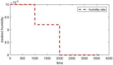
As mentioned before, the goal of control is to achieve the tracking to the desired temperature and humidity, Figures 2 and 3 plot the desired multilevel steps reference for humidity ratio and indoor temperature.
Figure 2. Desired humidity ratio
Figure 3. Desired indoor temperature
6.1 The open loop of AHU
In Figures 4 and 5 the open-loop response is plotted. The response demonstrated that the open the system is unstable and can’t follow the desirable thermal zone humidity ratio and air temperature. In fact, this result is mentioned in Remark (2) which explains the need to the control system.
Figure 4. Response of humidity u1&u2=0
Figure 5. Response of indoor temperature u1&u2=0
6.2 AHUs with 35% parameters variation
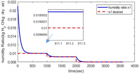
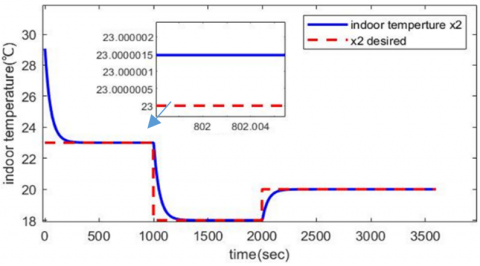
With the uncertainty in the system parameters listed in Table 4 by 35% from there nominal values, Figures 6 and 7 show the time response for both the thermal zone humidity ratio and air temperature by applying the proposed controllers. As can be seen, u1 is able to obtain the desired multilevel steps humidity ratio with very small error value (2.2*10-7) and acceptable settling time, while the second controller u2 which is ISMC based on barrier function coupled with LQR be able to obtain desired indoor air temperature with error value less than (1.47*10-6) and with small settling time.
Figure 6. Response of humidity ratio with 35% parameter variation
Figure 7. Response of indoor temperature with 35% parameters variation
Figure 8 plots the estimated e3 and the actual value with time. The performance of the ACSMD can be clarified from this figure where the main objective is to force the estimated state to pursue the actual one in a short time with smooth response. It is obvious that the steady-state error is equal to 5*10-4, according to Remark (4). After that, the estimated state ν will be used to build the sliding variable of the second controller.
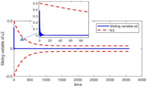
In Figures 9 and 10 are devoted to plot the integral sliding variables s1, s2. As can be seen from these figures, s1 & s2 are confined with ϵ1 and ϵ2 in $\forall t \geq 0$.
Figure 8. The estimation of e3
As can be seen that sliding variable did not exceed the ϵ1 value which is a constant value for the first controller, and ϵ2 which is a variable function for the second controller Eq. (46). The reason behind using variable ϵ2 can be seen in Figure 10, where high value of the second sliding variable can be absorbed using an appropriate large value of ϵ21. Also, ϵ2→ϵ22 after a period of time determined depending on the value of λ.
Figure 9. Sliding variable s1 vs. time
Figure 10. Sliding variable s2 vs. time
Figures 11 and 12 demonstrated the control signals where the ISMC based on barrier function which can effectively overcome the coupling control problem and compensate the uncertainty as well as compensate the disturbance, like when the second controller u2 compensates u1, since it is considered as external disturbance without need to prior information about upper bound of uncertainty and disturbance. Also, the chattering effect is eliminated because barrier function is a continuous function as mentioned in Remark 6.
Eventually it can be seen that optimal linear control strategy is effective strategy to enhance the ISMC to have a better performance.
Figure 11. Air flow rate u1
Figure 12. Water flow rate u2
To investigate the benefit of using optimal ISMC based in barrier function, Figure 13 shows the response of the indoor temperature by using ISMC based on barrier function and optimal ISMC based also on barrier function. The plot illustrates that the ISMC based on barrier function forced the indoor temperature to follow the desired temperature with steady state error less than 1.5*10-9 and with less settling time compared with ISMC uses the LQR technique, but with increasing in water flow rate u2 as seen in Figure 14 which leads to increase the energy consumption.
Figure 13. Response of indoor temperature with 35% parameters variation
Figure 14. Water flow rate u2
6.3 AHUs with 50% parameters variation
To prove the robustness and tracking of humidity ratios and indoor temperature, different uncertainty percent is examined. Figures 15 and 16 illustrate the time response of output states respectively with 50% of system parameter variation. It can be observed that proposed controllers can efficiently achieve rejection of the external disturbance, robustness and desired tracks to the required humidity ratio and indoor for the temperature with steady state error less than 2.5*10-7 and 1.47*10-6, respectively.
Figure 15. Response of humidity ratio with 50% parameter variation
Figure 16. Response of indoor humidity with 50% parameter variation
This paper presented AHUs which had muti-input multi-output. Two control strategy was proposed to achieve robustness and desired tracking. Firstly, the Integral sliding mode based on barrier function for the first control was proposed which was combined the properties of the ISMC and the barrier function. The main advantages of this strategy are the elimination of reaching phase and overcoming the problem of requiring knowing the upper bounds on the system parameters variation and on the disturbance to compute the discontinues gain and that by using the barrier function instead of the discontinuous control term. At the same time the chattering was eliminated because the control law is continuous and differentiable function which is essential property in designing the second controller.
The second control was couple ISMC based on barrier function and optimal feedback control using LQR. The proposed controller can effectively compensate the uncertainties, eliminate the chattering effect and provide the optimal performance of the linear control term. Finally, to overcome the problem of unmeasurable state an ACSMD was used which it is an impressive choice that proved robustness and accurate result in estimating the time derivative of the second error state which is used to form the sliding variable of the second controller. The numerical simulation was used to examine the performance of the proposed controllers with 35%, and 50% variation in the system parameters from their nominal values which are listed in Table 4. The results demonstrated clearly that the ISMC based on barrier function can assure robustness from the first and during an entire system response and can achieve tracking with a small steady state error for both humidity ratio and indoor temperature.
[1] Unde1rwood, C.P. (1999). HVAC Control Systems: Modeling, Analysis and Design. E & FN Spon, London and New York. https://doi.org/10.4324/9780203028704
[2] Afroz, A., Shafiullah, G., Urmee, T., Higgins, G. (2017). Modeling techniques used in building control systems: A review. Renewable and Sustainable Energy Reviews, 83: 64-84. https://doi.org/10.1016/j.rser.2017.10.044
[3] Yao, Y., Yeubin, Y. (2017). Modeling and Control in Air-Conditioning Systems, Energy and Environment Research in China. Springer Berlin, Heidelberg.
[4] Razban, A., Khatib, A., Goodman, D., Chen, J. (2019). Modelling of air handling unit subsystem in a commercial building. Thermal Science and Engineering Progress, 11: 231-238. https://doi.org/10.1016/j.tsep.2019.03.019
[5] Attaran, S.M., Yusof, R., Selamat, H. (2014). Decoupled HAVC system via non-linear decoupling algorithm to control the parameters of humidity and temperature through the adaptive controller. International Journal of Scientific and Research Publications, 4(4): 2250-3153.
[6] Ganchev, I., Taneva, A., Kutryanski, K., Petrov, M. (2019). Decoupling fuzzy-neural temperature and humidity control in HVAC systems. IFAC PapersOnLine, 52(25): 299-304. https://doi.org/10.1016/j.ifacol.2019.12.539
[7] Yuan, S., Zhang, L., Holub, O., Baldi., S. (2018) Switched adaptive control of air handling units with discrete and saturated actuators. IEEE Control Systems Letters, 2(3): 417-422. https://doi.org/10.1109/lcsys.2018.2840041
[8] Seong, N.C., Kim, J.H., Choi, W. (2019). Optimal control strategy for variable air volume air-conditioning systems using genetic algorithms. Sustainability, 11(18): 5122. https://doi.org/10.3390/su11185122
[9] Shah, A., Huang, D. Chen, Y., Kang, X., Qin, A. (2017). Robust sliding mode control of air handling unit for energy efficiency enhancement. Energies, 10(11): 1815. https://doi.org/10.3390/en10111815
[10] Shah, A., Huang, D., Huang, T. (2020). Dynamic modelling and multivariable control of buildings climate by using sliding mode control. 2020 IEEE International Conference on Artificial Intelligence and Information Systems (ICAIIS), Dalian, China, pp 552-555. https://doi.org/10.1109/ICAIIS49377.2020.9194861
[11] Setayesh, H., Moradi, H., Alasty, A. (2019). Nonlinear robust control of air handling units to improve the indoor air quality & CO2 concentration: A comparison between H∞ & decoupled sliding mode controls. Applied Thermal Engineering, 160: 113958. https://doi.org/10.1016/j.applthermaleng.2019.113958
[12] Niu, F., Li, Z., Yang, L., Wu, Z., Zhu, Q., Jiang, B. (2020). Fuzzy sliding mode control of a VAV air-conditioning terminal temperature system. Complexity, 2020: 8823674. https://doi.org/10.1155/2020/8823674
[13] Hassan, M.R., Al-Samarraie, S.A. (2022). Robust nonlinear control design for the HVAC system based on adaptive sliding mode control. Journal Européen des Systèmes Automatisés, 55(5): 593-601. https://doi.org/10.18280/jesa.550504
[14] Barambones, O., Garrido, A.J., Maseda, F.J. (2007). Integral sliding-mode controller for induction motor based on field-oriented control theory. IET Control Theory & Applications, 1(3): 786-794. https://doi.org/10.1049/iet-cta:20060239
[15] Rubagotti, M., Estrada, A., Castaños, F., Ferrara, A., Member, S., Fridman, L. (2011). Integral sliding mode control for nonlinear systems with matched and unmatched perturbations. IEEE Transaction on Automatic Control, 56(11): 2699-2704. https://doi.org/10.1109/TAC.2011.2159420
[16] Al-Samarraie, S.A., Badri, A., Mshari, M.H. (2015). Integral sliding mode control desfor electronic throttle valve system. Engineering Journal, 11(3): 72-84.
[17] Abd, A.F., Al-Samarraie, S.A. (2021). Integral sliding mode control based on barrier function for servo actuator with friction. Engineering and Technology Journal, 39(2A): 248-259. http://dx.doi.org/10.30684/etj.v39i2A.1826
[18] Husain, S.S., Ridha, T.M. (2022). Design of integral sliding mode control for seismic effect regulation on buildings with unmatched disturbance. Mathematical Modelling of Engineering Problems, 9(4): 1123-1130. https://doi.org/10.18280/mmep.090431
[19] Jouini, M., Dhahri, S., Sellami, A. (2018). Combination of integral sliding mode control design with optimal feedback control for nonlinear uncertain systems. Transaction of the Institute of Measurement and Control, 41(5): 1-9. https://doi.org/10.1177/0142331218777562
[20] Xu, X., Zhong, Z., Deng, S., Zhang, X.(2017). A review on temperature and humidity control methods focusing on air-conditioning equipment and control algorithms applied in small-to-medium-sized buildings. Energy and Buildings, 162: 163-176. https://doi.org/10.1016/j.enbuild.2017.12.038
[21] Shah, Z.A., Sind, H.F., Ul-haq, A., Ali, M.A. (2020). Fuzzy logic-based direct load control scheme for air conditioning load to reduce energy consumption. IEEE Access, 8: 117413-117427. https://doi.org/10.1109/ACCESS.2020.3005054
[22] Jahedi, G., Ardehali, M.M. (2012). Wavelet based artificial neural network applied for energy efficiency enhancement of decoupled HVAC system. Energy Conversion and Management, 54(1): 47-56. https://doi.org/10.1016/j.enconman.2011.10.005
[23] Utkin, V., Guldner, J., Shi, J. (2009). Sliding Mode Control in Electro-Mechanical Systems. Taylor & Francis Group, LLC, 2nd edition. https://doi.org/10.1201/9781420065619
[24] Ezzaldean1, M.M., Kadhem, Q.S. (2019). Design of control system for 4-switch BLDC motor based on sliding-mode and hysteresis controllers. IJCCCE,19(1): 42-51. https://doi.org/10.33103/uot.ijccce.19.1.6
[25] Majeed, H.S., Kadhim, S.K., Jaber, A.A. (2022). Design of a sliding mode controller for a prosthetic human hand’s finger. Engineering and Technology Journal, 40(1): 257-266 http://dx.doi.org/10.30684/etj.v40i1.1943
[26] Obeid, H., Fridman, L.M., Laghrouche, S., Harmouche, M. (2018). Barrier function-based adaptive sliding mode control. Automatica, 93: 540-544. https://doi.org/10.1016/j.automatica.2018.03.078
[27] Utkin, V., Shi, J. (1996). Integral sliding mode in systems operating under uncertainty conditions. Proceedings of 35th IEEE Conference on Decision and Control, Kobe, Japan, pp. 4591-4596. https://doi.org/10.1109/CDC.1996.577594
[28] Lui, Z., Pan, H. (2021). Barrier function-based adaptive sliding mode control for application to vehicle suspensions. IEEE Transactions on Transportation Electrification, 7(3): 2023-2033. https://doi.org/10.1109/TTE.2020.3043581
[29] Dorf, R.C. (2003). Optimal Control System. New York: CRC Press LLC.
[30] Inman, D.J. (2006). Vibration with Control. USA: John Wiley & Sons Ltd.
[31] Das, S., Pan, I., Halder, K., Das, S., Gupta, A. (2013). Optimum weight selection based LQR formulation for the design of fractional order PIλDμ controllers to handle a class of fractional order systems. 2013 International Conference on Computer Communication and Informatics, Coimbatore, India, pp. 1-6. https://doi.org/10.1109/ICCCI.2013.6466137
[32] Prasad L.B., Tyagi B., Gupta H.O. (2014). Optimal control of nonlinear inverted pendulum system using PID controller and LQR: Performance analysis without and with disturbance input. International Journal of Automation and Computing, 11(6): 661-670. https://doi.org/10.1007/s11633-014-0818-1
[33] Al-Samarraie S.A. (2013). Invariant sets in sliding mode control theory with application to servo actuator system with friction. WSEAS Transactions on Systems and Control, 8(2): 33-45.
[34] Al-Samarraie, S.A., Mishary, M.H. (2018). A chattering free sliding mode observer with application to DC motor speed control. 2018 Third Scientific Conference of Electrical Engineering (SCEE), Baghdad, Iraq, pp. 259-264. https://doi.org/10.1109/SCEE.2018.8684128
[35] Humaidi, A.J., Hameed, A.H., Ibraheem, I.K. (2019). Design and performance study of two sliding mode backstepping control schemes for roll channel of delta wing aircraft. 019 6th International Conference on Control, Decision and Information Technologies (CoDIT), Paris, France, pp. 1215-1220. https://doi.org/10.1109/CoDIT.2019.8820315