Layla Hindi*![]() | Hussein K. Asker
| Hussein K. Asker![]()
© 2023 IIETA. This article is published by IIETA and is licensed under the CC BY 4.0 license (http://creativecommons.org/licenses/by/4.0/).
OPEN ACCESS
The safety and availability of cold standby systems are often critically dependent on the successful activation and subsequent operation of their standby components. In this study, an availability estimation model is developed for a repairable 1-out-of-3 cold standby system and applied to a real industrial scenario involving a main electrical power network, a local electricity generator, and a domestic electricity generator. A repairable 1-out-of-3 cold standby system comprising three components is evaluated, and Markov models for system reliability are introduced. The analysis reveals a relatively high availability, indicating that the main electrical power network (MEPN) is essential. Furthermore, the effects of component capacity partitioning on system availability are investigated through numerical analysis. The results demonstrate that a 1-out-of-3 system exhibits improved performance and stability due to its higher capacity level.
1-out-of-3 cold standby system, markov model, steady-state availability
System availability is of paramount importance for operations under challenging environments. In the digital economy, critical facilities such as data centers, communication centers, and financial services necessitate continuous, high-quality electrical supplies. To ensure exceptional availability, the power supply must be extremely reliable [1]. The main electrical power network (MEPN) in Iraq plays a vital role in daily life, powering various electrical tools that make life more convenient. However, due to frequent blackouts in the MEPN, people have turned to private generators, either local ones that supply power to each block or domestic ones used in individual households. Although these generators present their own challenges, they serve as essential alternatives during extensive blackouts in the MEPN. Consequently, these three power sources operate in tandem, with repair processes required when their functionality falters. This leads to part-time operation availability for the system. Achieving the desired level of availability involves providing sufficient redundancy, reducing the probability of failure, and minimizing repair time [2]. Availability is contingent upon the types of breakdowns included in the analysis [3].
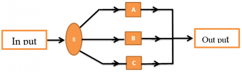
Redundancy is a valuable tool for enhancing a system's availability by adding plug-ins. The plug-ins' status determines the type of redundancy, which can be classified into active redundancy, standby redundancy, and active/standby redundancy. Standby redundancy systems are configurations where a system is considered to have failed when all units have failed. In such systems, only one unit (or a defined number) operates at a time, while the other units await activation upon the operating unit's failure [4], as illustrated in Figure 1. This system comprises three units: A represents the initially operating unit, B and C are standby units, and S is the changeover device (switch). Standby systems can be further classified into cold standby, hot standby, and warm standby [5].
Figure 1. 1-out-of-3 standby system
This study focuses on cold standby systems. In such systems, the standby units do not carry any load during the waiting period before activation. They remain in a dormant mode with a zero failure rate, while active units experience a higher failure rate of () [2, 4]. A comprehensive literature review reveals various studies examining the advantages and characteristics of cold standby systems.
Chung [6] clarified that active and cold standby units exhibit different constant failure rates, with failed system repair times having arbitrary distributions. Asker [4] investigated a two-unit repairable standby system with a changeover device (switch) functioning either perfectly or imperfectly, in conjunction with a cold or partly loaded standby unit, resulting in eight distinct models for the system. Wang and Loman [1] proposed a generalized repairable system reliability model, K-out-of-N, with M cold standby units, which was subsequently applied by the General Electric Company to design an on-site power plant with N active generators (operating in de-rating mode) and backup generators in standby. This design aimed to provide an extremely reliable power source. Pérez-Ocón and Montoro-Cazorla [7] presented a system comprising n units, with only the working unit being susceptible to failure, while the other units are in repair, cold standby, or waiting for repair.
Zhang and Wang [8] examined a two-component cold standby repairable system with one repairman and the use of priority, assuming that component M after repair is not "as good as new". Manglik and Ram [9] analyzed the reliability of a four-component system arranged in series, where subsystems A, B, and C consist of single units, and subsystem D comprises three units: one active and two in cold standby arranged in parallel. Bao and Cui [10] proposed a new repairable system based on a Markov repairable two-item cold standby system, in which the effects of system failure could be neglected. Zhai et al. [11] explored a 1-out-of-n cold standby system, scheduling backups to ensure a standby component can effectively take over the task when the online component fails.
Grida et al. [2] addressed the effects of plug-in economy of scale on achieving high availability levels. Peng et al. [12] investigated a cold standby system with two different components, utilizing the highly applicable phase-type (PH) distribution to describe the life and maintenance time of system components in a unified manner and constructing a systems' reliability model for broader applicability. Batra et al. [13] optimized the number of standby units for a system with one operative unit, using Semi-Markov processes and the regenerative point technique. Krishnan [14] provided a survey of reliability studies on k-out-of-n: G systems, exploring various cases and applications. Grida et al. [15] employed the Markov modeling technique to compute the reliability and mean time to failure for non-repairable systems with varying failure rates.
Savita et al. [16] conducted a study on a system with two distinct units, one of good quality and another of substandard quality, analyzing the system to determine reliability measures using the Semi-Markov process and the Regenerative technique. Ruiz-Castro [17] examined matrix analysis methods for modeling complex discrete cold standby systems subject to multiple events, facilitating algorithmic and computational development of multi-state complex systems. The presented method enabled the analysis of optimization problems in multi-state complex systems, providing results that demonstrate the profitability of preventive maintenance and revealing the optimal number of operational units. Patawa et al. [18] analyzed the behavior of two dissimilar units in a cold standby repairable system with a waiting time facility, establishing that the Bayesian method under suitable prior is a practical and straightforward approach for analyzing redundant repairable systems with a waiting time facility. Danjuma et al. [19] investigated the reliability of a system with three components (A, B, and C) coupled in series and parallel, evaluating the system using the Markov birth-death process and deriving expressions for availability and mean time to system breakdown. The results indicated that system effectiveness indicators, such as availability and mean time to system failure, increase with repair rates and decrease with failure rates.
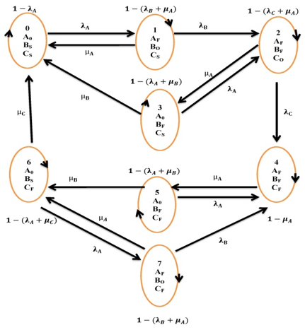
In light of these studies and frequent outages in the Main Electrical Power Network (MEPN) in Iraq, which has led to the reliance on local and domestic electricity generators, this paper evaluates a cold standby system model of 1-out-of-3. The system comprises three components representing the main electrical power network, a local generator, and a domestic generator. The 1-out-of-3 cold standby system prioritizes the use and maintenance of components, with the backup itself being a 1-out-of-3 system. A set of assumptions, including cold standby, perfect switching, and a 1-out-of-3 system for the backup, are considered. The entire process is demonstrated and explained using a Markov Transition Chart, as shown in Figure 2.
The remainder of the paper is organized as follows: Section 2 provides a detailed description of the considered system. Section 3 describes the system state using the transition matrix. Section 4 presents the availability of the two cold standby systems with repairable components and calculates the stationary availability of the system. Section 5 examines the effect of component capacity partitioning on system availability for a 1-out-of-3 cold standby system. Finally, Section 6 discusses the findings and offers conclusions.
Figure 2. Markov transition diagram for 1-out-of -3 cold standby system
In the current study, we have evaluated a repairable 1-out-of-3 cold standby system, which comprises of three components: A is the initial operational component, B, C are the two cold standby components. As shown, component A is the (MEPN), component B is the local power generator, and component C is the household electricity generator. The assumptions are detailed as follows:
1. The switching of the system to be perfect. Hence, failure of the active component A is detected immediately, and B standby component is activated with probability 1 (It does not fail during its operation and does not fail in switching from normal operating component to the standby component).
2. At the beginning of the operation of the system, component A starts operation first, if it is in a good state while the components B and C in standby state.
3. Component A has priority in use and maintenance, and components B and C are repaired sequentially. In other words when component A is satisfactorily repaired when component B is in service state, component B is replaced by it. So component A enters the service state, and component B enters the standby state or fails.
4. When a component fails, it is instantaneously replaced by one of the standby components.
5. Each component has a constant operating failure rate (λ), and a constant repair rate (μ).
6. The time of repair is exponentially distributed with repair rate (μ).
7. When repair action is completed, component A is placed in operating state and the components B and C are placed in standby state.
8. System failure occurs when the operating component A fails before repairing the other components B or C.
9. The failed state of the system is state (4) as shown in Figure 2, when all components have failed, one of them is repaired instantaneously, which is (A) and the system is thus transitioned to state (5).
The transition of a system from one state to another is best described by the transition matrix, as in Table 1.
Using the time derivative of state probabilities and a Markov transition diagram to examine the system states depicted in Figure 2 and Table 1, we can construct the following formulas as the state probabilities of the system.
Table 1. Transition probability matrix
|
|
P0 |
P1 |
P2 |
P3 |
P4 |
P5 |
P6 |
P7 |
|
P0 |
- λA |
λA |
0 |
0 |
0 |
0 |
0 |
0 |
|
P1 |
µA |
- (λB+ µA) |
λB |
0 |
0 |
0 |
0 |
0 |
|
P2 |
0 |
0 |
- (λC+ µA) |
µA |
λC |
0 |
0 |
0 |
|
P3 |
µB |
0 |
λA |
- (λA+ µB) |
0 |
0 |
0 |
0 |
|
P4 |
0 |
0 |
0 |
0 |
- µA |
µA |
0 |
0 |
|
P5 |
0 |
0 |
0 |
0 |
λA |
- (λA+ µB) |
µB |
0 |
|
P6 |
µC |
0 |
0 |
0 |
0 |
0 |
- (λA+ µC) |
λA |
|
P7 |
0 |
0 |
0 |
0 |
λB |
0 |
µA |
- (λB+ µA) |
$\frac{d p_1(t)}{d t}=\lambda p_0-(\lambda+\mu) p_1$, (2)
$\frac{d p_2(t)}{d t}=\lambda p_1-(\lambda+\mu) p_2+\lambda p_3$, (3)
$\frac{d p_3(t)}{d t}=\mu p_2-(\lambda+\mu) p_3$, (4)
$\frac{d p_4(t)}{d t}=\lambda p_2-\mu p_4+\lambda p_5+\lambda p_7$, (5)
$\frac{d p_5(t)}{d t}=\lambda p_4-(\lambda+\mu) p_5$, (6)
$\frac{d p_6(t)}{d t}=\mu p_5-(\lambda+\mu) p_6+\mu p_7$, (7)
$\frac{d p_7(t)}{d t}=\lambda p_6-(\lambda+\mu) p_7$. (8)
Under steady state, the time derivatives of state probability are:
$p_0=\left[\frac{\lambda+\mu}{\lambda}\right] p_1$, (9)
$p_2=\left[\frac{\lambda(\lambda+\mu)}{\lambda^2+\lambda \mu+\mu^2}\right] p_1$, (10)
$p_3=\left[\frac{\lambda \mu}{\lambda^2+\lambda \mu+\mu^2}\right] p_1$, (11)
$\begin{aligned} p_4=\left[2 \frac{\lambda^2}{\mu^2}+\frac{\lambda^3}{\mu^3}\right. & -\frac{\lambda^3}{\mu^3+\lambda \mu^2}-\frac{2 \lambda^2-\lambda \mu}{\lambda^2+\lambda \mu+\mu^2}-\frac{\lambda^3}{\lambda^2 \mu+\lambda \mu^2+\lambda^3}+\frac{\lambda}{\mu}-\frac{\lambda^2}{\mu^2+\lambda \mu} \left.+\frac{\lambda^3+\lambda^2 \mu}{\lambda^3+2 \lambda^2 \mu+2 \lambda \mu^2+\mu^3}\right] p_1\end{aligned}$, (12)
$p_5=\left[\frac{\lambda^2}{\mu^2}-\frac{\lambda^2-\lambda \mu}{\lambda^2+\lambda \mu+\mu^2}+\frac{\lambda}{\mu}-\frac{\lambda^2}{\lambda \mu+\mu^2}+\frac{\lambda^2 \mu}{\lambda^3+2 \lambda^2 \mu+2 \lambda \mu^2+\mu^3}\,\,\right] p_1$, (13)
$p_6=\left[\frac{\lambda}{\mu}-\frac{\lambda \mu}{\lambda^2+\lambda \mu+\mu^2}\right] p_1$, (14)
$p_7=\left[\frac{\lambda^2}{\lambda \mu+\mu^2}-\frac{\lambda^2 \mu}{\lambda^3+2 \lambda^2 \mu+2 \lambda \mu^2+\mu^3}\,\,\right] p_1$, (15)
Combining Eqns. (9)-(15) and condition
$\sum_{i=0}^7 p_i(t)=1$ (16)
$p_1=\frac{\lambda \mu^3}{\lambda^4+2 \lambda^3 \mu+2 \lambda^2 \mu^2+2 \lambda \mu^3+\mu^4}$ , (17)
So
$p_0=\frac{\mu^3(\lambda+\mu)}{\lambda^4+2 \lambda^3 \mu+2 \lambda^2 \mu^2+2 \lambda \mu^3+\mu^4}$ , (18)
$p_2=\frac{\lambda^2 \mu^3(\lambda+\mu)}{\left(\lambda^2+\lambda \mu+\mu^2\right)\left(\lambda^4+2 \lambda^3 \mu+2 \lambda^2 \mu^2+2 \lambda \mu^3+\mu^4\right)}$ , (19)
$p_3=\frac{\lambda^2 \mu^3}{\left(\lambda^2+\lambda \mu+\mu^2\right)\left(\lambda^4+2 \lambda^3 \mu+2 \lambda^2 \mu^2+2 \lambda \mu^3+\mu^4\right)}$ , (20)
$\begin{gathered}p_4=\frac{\lambda^4+2 \lambda^3 \mu+\lambda^2 \mu^2}{\left(\lambda^4+2 \lambda^3 \mu+2 \lambda^2 \mu^2+2 \lambda \mu^3+\mu^4\right)} \\ -\frac{\lambda^4 \mu^3}{\left(\lambda^2 \mu+\lambda \mu^2+\mu^3\right)\left(\lambda^4+2 \lambda^3 \mu+2 \lambda^2 \mu^2+2 \lambda \mu^3+\mu^4\right)}-\frac{\lambda^3 \mu^3}{\left(\mu^2+\lambda \mu\right)\left(\lambda^4+2 \lambda^3 \mu+2 \lambda^2 \mu^2+2 \lambda \mu^3+\mu^4\right)} \\ -\frac{\lambda^4\mu^3}{\left(\mu^3+\lambda \mu^2\right)\left(\lambda^4+2 \lambda^3 \mu+2 \lambda^2 \mu^2+2 \lambda \mu^3+\mu^4\right)} \\ +\frac{\lambda^3 \mu^4+\lambda^4 \mu^3}{\left(\lambda^3+2 \lambda^2 \mu+2 \lambda \mu^2+\mu^3\right)\left(\lambda^4+2 \lambda^3 \mu+2 \lambda^2 \mu^2+2 \lambda \mu^3+\mu^4\right)} \\ -\frac{\lambda^2 \mu^3-2 \lambda^3 \mu^3}{\left(\lambda^2+\lambda \mu+\mu^2\right)\left(\lambda^4+2 \lambda^3 \mu+2 \lambda^2 \mu^2+2 \lambda \mu^3+\mu^4\right)}\end{gathered}$, (21)
$\begin{gathered}p_5=\frac{\lambda^3 \mu+\lambda^2 \mu^2}{\left(\lambda^4+2 \lambda^3 \mu+2 \lambda^2 \mu^2+2 \lambda \mu^3+\mu^4\right)}-\frac{\lambda^3 \mu^3}{\left(\mu^2+\lambda \mu\right)\left(\lambda^4+2 \lambda^3 \mu+2 \lambda^2 \mu^2+2 \lambda \mu^3+\mu^4\right)} \\ +\frac{\lambda^3 \mu^4}{\left(\lambda^3+2 \lambda^2 \mu+2 \lambda \mu^2+\mu^3\right)\left(\lambda^4+2 \lambda^3 \mu+2 \lambda^2 \mu^2+2 \lambda \mu^3+\mu^4\right)} \\ -\frac{\lambda^2 \mu^3-2 \lambda^3 \mu^3}{\left(\lambda^2+\lambda \mu+\mu^2\right)\left(\lambda^4+2 \lambda^3 \mu+2 \lambda^2 \mu^2+2 \lambda \mu^3+\mu^4\right)}\end{gathered}$, (22)
$p_6=\frac{\lambda^2 \mu^2}{\left(\lambda^4+2 \lambda^3 \mu+2 \lambda^2 \mu^2+2 \lambda \mu^3+\mu^4\right)}-\frac{\lambda^2 \mu^4}{\left(\lambda^2+\lambda \mu+\mu^2\right)\left(\lambda^4+2 \lambda^3 \mu+2 \lambda^2 \mu^2+2 \lambda \mu^3+\mu^4\right)}$ , (23)
$p_7=\frac{\lambda^3 \mu^3}{\left(\lambda \mu+\mu^2\right)\left(\lambda^4+2 \lambda^3 \mu+2 \lambda^2 \mu^2+2 \lambda \mu^3+\mu^4\right)}-\frac{\lambda^3 \mu^4}{\left(\lambda^3+2 \lambda^2 \mu+2 \lambda \mu^2+\mu^3\right)\left(\lambda^4+2 \lambda^3 \mu+2 \lambda^2 \mu^2+2 \lambda \mu^3+\mu^4\right)}$ (24)
Availability is the probability that the system is operating at a specified time (t), which is always associated with the concept of maintainability. Availability depends on both failures and relies on repair rates [9].
4.1 Calculate the stationary availability of system
The system is in operation when it is in either the state $p_0$, $p_1$, $p_2$, $p_3$, $p_4$, $p_5$, $p_6$ and $p_7$. Therefor, the general form to calculate the stationary availability of system is:
$\begin{gathered}\mathrm{V}_{\mathrm{AA}}=\left[p_0(\infty)+p_1(\infty)+p_2(\infty)+p_3(\infty)\right. \left.+p_5(\infty)+p_6(\infty)+p_7(\infty)\right] .\end{gathered}$ (25)
Using Eqns. (17)-(20) and Eqns. (22)-(25) can be rewritten as:
$\begin{aligned} & \mathbf{V}_{\mathbf{A A}}=\left[\frac{\mu^3(\lambda+\mu)}{\lambda^4+2 \lambda^3 \mu+2 \lambda^2 \mu^2+2 \lambda \mu^3+\mu^4}+\frac{\lambda \mu^3}{\lambda^4+2 \lambda^3 \mu+2 \lambda^2 \mu^2+2 \lambda \mu^3+\mu^4}\right. \\ & +\frac{\lambda^2 \mu^3(\lambda+\mu)}{\left(\lambda^2+\lambda \mu+\mu^2\right)\left(\lambda^4+2 \lambda^3 \mu+2 \lambda^2 \mu^2+2 \lambda \mu^3+\mu^4\right)}+\frac{\lambda^2 \mu^4}{\left(\lambda^2+\lambda \mu+\mu^2\right)\left(\lambda^4+2 \lambda^3 \mu+2 \lambda^2 \mu^2+2 \lambda \mu^3+\mu^4\right)} \\ & +\frac{\lambda^3 \mu+\lambda^2 \mu^2}{\left(\lambda^4+2 \lambda^3 \mu+2 \lambda^2 \mu^2+2 \lambda \mu^3+\mu^4\right)}-\frac{\lambda^3 \mu^3}{\left(\mu^2+\lambda \mu\right)\left(\lambda^4+2 \lambda^3 \mu+2 \lambda^2 \mu^2+2 \lambda \mu^3+\mu^4\right)} \\ & +\frac{\lambda^3 \mu^4}{\left(\lambda^3+2 \lambda^2 \mu+2 \lambda \mu^2+\mu^3\right)\left(\lambda^4+2 \lambda^3 \mu+2 \lambda^2 \mu^2+2 \lambda \mu^3+\mu^4\right)} \\ & +\frac{\lambda^2 \mu^2}{\left(\lambda^4+2 \lambda^3 \mu+2 \lambda^2 \mu^2+2 \lambda \mu^3+\mu^4\right)} \\ & -\frac{\lambda^2 \mu^4}{\left(\lambda^2+\lambda \mu+\mu^2\right)\left(\lambda^4+2 \lambda^3 \mu+2 \lambda^2 \mu^2+2 \lambda \mu^3+\mu^4\right)} \\ & +\frac{\lambda^3 \mu^3}{\left(\lambda \mu+\mu^2\right)\left(\lambda^4+2 \lambda^3 \mu+2 \lambda^2 \mu^2+2 \lambda \mu^3+\mu^4\right)} \\ & \left.-\frac{\lambda^3 \mu^4}{\left(\lambda^3+2 \lambda^2 \mu+2 \lambda \mu^2+\mu^3\right)\left(\lambda^4+2 \lambda^3 \mu+2 \lambda^2 \mu^2+2 \lambda \mu^3+\mu^4\right)}\right] \\ & \end{aligned}$.
So,
$\mathrm{V}_{\mathrm{AA}}=\frac{\mu^4+2 \lambda \mu^3+\lambda^3 \mu+2 \lambda^2 \mu^2}{\lambda^4+2 \lambda^3 \mu+2 \lambda^2 \mu^2+2 \lambda \mu^3+\mu^4}$ (26)
Term (Γ) is defined as the ratio of repair rate to component failure rate and is used to analyze the impact of component capacity partitioning on system availability: $\Gamma=\mu / \lambda$.
Hence, we will calculate and analyze the effect of component capacity partitioning on system availability 1-out-of-3 cold standby system from Eq. (26).
$V_{A A}=\frac{\Gamma^4+2 \Gamma^3+\Gamma+2 \Gamma^2}{1+2 \Gamma+2 \Gamma^2+2 \Gamma^3+\Gamma^4}$ (27)
Taking the individual values of different (Γ) the ratio of repair rate to component failure rate and substitute into an Eq. (27). Table 2 shows the availability values.
Table 2. Calculates the availability
|
Γ values |
VAA values |
||
|
Γ 1 |
1 |
VAA1 |
0.7500000 |
|
Γ 2 |
1.5 |
VAA2 |
0.87692307 |
|
Γ 3 |
11 |
VAA3 |
0.9993169 |
|
Γ 4 |
21 |
VAA4 |
0.9998971 |
|
Γ 5 |
31 |
VAA5 |
0.9999675 |
|
Γ 6 |
41 |
VAA6 |
0.9999858 |
|
Γ 7 |
51 |
VAA7 |
0.9999926 |
|
Γ 8 |
61 |
VAA8 |
0.9999956 |
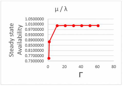
Figure 3. The steady state availability with respect to components setting up and Γ
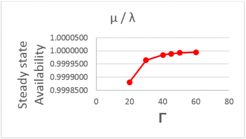
Taking the marital values of different (Γ) the ratio of repair rate to component failure rate and substitute into an Eq. (27). And we get Table 3 to see the availability values.
The following chart shows the values of the second table graphically,
Figure 4. The steady state availability with respect to components setting up and Γ
Table 3. Calculates the availability
|
Γ values |
VAA values |
||
|
Γ 1 |
20 |
VAA1 |
0.9998812 |
|
Γ 2 |
30 |
VAA2 |
0.9999641 |
|
Γ 3 |
40 |
VAA3 |
0.9999847 |
|
Γ 4 |
50 |
VAA4 |
0.9999921 |
|
Γ 5 |
60 |
VAA5 |
0.9999954 |
In this paper, we have a model for a 1-out-of-3 cold standby system developed and studied on the real industrial application of the (MEPN), local electricity generator and domestic electricity generator. Various reliability indices are evaluated such as availability for the considered system by employing Markov Process. From the results and analysis of the designed system, one can conclude the following:
(i) Figure 3 and Figure 4 show the expected stable availability of a 1-out-of-3 cold standby system. In terms of repair failure rate, a 1-out-of-3 system performed better due to its higher level of redundancy. To have a higher repair failure rate, the performance of 1-out-of-3 is better.
(ii) The analysis of the models shown have relatively high availability according to the model and that the (MEPN) cannot be dispensed with.
I would like to acknowledge and give my warmest thanks to my supervisor (Dr. Hussein K. Asker) who made this work possible. His guidance and advice carried me through all the stages of writing my paper.
Matlab (R2014a) was used in the current study to examine the results of all the formulas mentioned above. Moreover, the (R2014a) software was used to draw the diagrams (3A and 3B).:
Code Matlab
P00=solve("X∗P0−(X+Y)∗P1=0","P0")
P22=solve(′Y∗P2−(X+Y)∗P3=0"," P2")
P33=X∗P1−(X+Y)∗P22+X∗P3
P333=solve(P33," P3")
P222=subs(P22, P3, P333)
P66=solve("−X∗P0+Y∗P1+Y∗P3+Y∗P6=0","P6")
P666=subs(P66, P3, P333)
P6666=expand(subs(P666, P0, P00))
P77=solve(′X∗P6−(X+Y)∗P7=0′," P7")
P777=expand(subs(P77, P6, P6666))
P55=solve("Y∗P5−(X+Y)∗P6+Y∗P7=0","P5")
P555=subs(P55, P6, P6666)
P5555=expand(subs(P555, P7, P777))
P44=solve("Y∗P4−(X+Y)∗P5"," P4")
P444=expand(subs(P44, P5, P5555))
P11=P00+P1+P222+P333+P444+P5555+P6666+P777
P111=solve(P11=1,P1)
PP0=subs(P00,P1,P111)
PP2=subs(P222,P1,P111)
PP3=subs(P333,P1,P111)
PP4=subs(P444,P1,P111)
PP5=subs(P5555,P1,P111)
PP6=subs(P6666,P1,P111)
PP7=subs(P777,P1,P111)
KKK=PP0+P111+PP2+PP3+PP5+PP6+PP7
KKK2=expand(PP0+P111+PP2+PP3+PP5+PP6+PP7)
KKK3=expand(KKK2+PP4)
P44444=1-PP4
clear all;clc;
X=[20 30 40 50 60]
Y=(X.4+2.∗(X.3)+X+2.∗(X.2))./(1+2.∗X+2.∗(X.2)+2.∗(X.3)+(X.4))
plot(X, Y)
X=[1 1.5 11 21 31 41 51 61]
Y=(X.4+2.∗(X.3)+X+2.∗(X.2))./(1+2.∗X+2.∗(X.2)+2.∗(X.3)+(X.4))
plot(X, Y)
[1] Wang, W., Loman, J. (2002). Reliability/availability of K-out-of-N system with M cold standby units. In Annual Reliability and Maintainability Symposium. 2002 Proceedings (Cat. No. 02CH37318). IEEE, pp. 450-455. https://doi.org/10.1109/RAMS.2002.981684
[2] Grida, M., Zaid, A., Kholief, G. (2017). Repairable 3-out-of-4: Cold standby system availability. In 2017 Annual Reliability and Maintainability Symposium (RAMS). IEEE, pp. 1-6. https://doi.org/10.1109/RAM.2017.7889797
[3] Bentley, J.P. (1999). Introduction to reliability and quality engineering. Prentice Hall.
[4] Asker, H.K. (2000). Reliability models for maintained and non-maintained systems. Master's Thesis. Mustansiriyah University.
[5] Wang, W., Kececioglu, D.B. (2000). Confidence limits on the inherent availability of equipment. In Annual Reliability and Maintainability Symposium. 2000 Proceedings. International Symposium on Product Quality and Integrity (Cat. No. 00CH37055). IEEE, pp. 162-168. https://doi.org/10.1109/RAMS.2000.816301
[6] Chung, W.K. (1984). A k-out-of-N: G redundant system with cold standby units and common-cause failures. Microelectronics Reliability, 24(4): 691-695. https://doi.org/10.1016/0026-2714(84)90218-X
[7] Pérez-Ocón, R., Montoro-Cazorla, D. (2004). A multiple system governed by a quasi-birth-and-death process. Reliability Engineering & System Safety, 84(2): 187-196. https://doi.org/10.1016/j.ress.2003.10.003
[8] Zhang, Y.L., Wang, G.J. (2007). A deteriorating cold standby repairable system with priority in use. European Journal of Operational Research, 183(1): 278-295. https://doi.org/10.1016/j.ejor.2006.09.075
[9] Manglik, M., Ram, M. (2013). Reliability analysis of a two unit cold standby system using markov process. Journal of Reliability and Statistical Studies, 65-80.
[10] Bao, X., Cui, L. (2012). A study on reliability for a two-item cold standby markov repairable system with neglected failures. Communications in Statistics-Theory and Methods, 41(21): 3988-3999. https://doi.org/10.1080/03610926.2012.700376
[11] Zhai, Q., Xing, L., Peng, R., Yang, J. (2015). Reliability analysis of cold standby system with scheduled backups. In 2015 Annual Reliability and Maintainability Symposium (RAMS). IEEE, pp. 1-6. https://doi.org/10.1109/RAMS.2015.7105121
[12] Peng, D., Zichun, N., Bin, H. (2018). A new analytic method of cold standby system reliability model with priority. In MATEC Web of Conferences. EDP Sciences, 175: 03060. https://doi.org/10.1051/matecconf/201817503060
[13] Batra, S., Taneja, G. (2018). Reliability and optimum analysis for number of standby units in a system working with one operative unit. International Journal of Applied Engineering Research, 13(5): 2791-2797.
[14] Krishnan, R. (2020). Reliability analysis of k-out-of-n: G system: A short review. International Journal of Engineering and Applied Sciences (IJEAS), 7: 21-24.
[15] Grida, S., Manglik, T., Taneja, S.U. (2020). Reliability and availability for non-repairable & repairable systems using markov modelling. International Journal of Engineering Research & Technology (IJERT). This Work is Licensed Under a Creative Commons Attribution 4.0 International License, 9(2): 628-634. ISSN: 2278-0181.
[16] Savita, P.B., Sanjeev, K. (2019). Reliability analysis of a redundant system with repair/replacement of cold standby unit. International Journal of Quality & Reliability Management, 36(6): 1053-1072.
[17] Ruiz-Castro, J.E. (2021). Optimizing a multi-state cold-standby system with multiple vacations in the repair and loss of units. Mathematics, 9(8): 913. https://doi.org/10.3390/math9080913
[18] Patawa, R., Pundir, P.S., Sigh, A.K., Singh, A. (2022). Some inferences on reliability measures of two-non-identical units cold standby system waiting for repair. International Journal of System Assurance Engineering and Management, 1-17. https://doi.org/10.1007/s13198-021-01188-7
[19] Danjuma, M.U., Yusuf, B., Ali, U.A., Ismail, A.L., Soltani, S., Sobhani, F.M., Najafi, S.E. (2022). Analysis of mean time to system failure and availability of a system with cold standby unit. Journal of Industrial Engineering International, 18(1): 2.