Bui Huy Hai![]()
© 2023 IIETA. This article is published by IIETA and is licensed under the CC BY 4.0 license (http://creativecommons.org/licenses/by/4.0/).
OPEN ACCESS
The Independent Component Analysis (ICA) method has been demonstrated as an effective tool for separating desired signals and artifacts in the processing of biomedical signals, particularly in electrocardiogram (ECG) recordings through blind source separation (BSS). Unwanted components, which propagate through the body to the electrodes and mix with the recorded signal, are analyzed into independent components (ICs). However, the unwanted ICs identified as artifacts may also contain valuable information, resulting in a loss of information if these ICs are removed entirely. To address this issue, a combined solution of wavelet decomposition and ICA is proposed. Wavelet decompositions are performed on the unwanted ICs, and the application of a threshold level to the wavelet coefficients minimizes the loss of information in the received signal. A proposed solution utilizing the wavelet-based ICA (wICA) algorithm effectively removes artifacts, reducing distortion in the amplitude and phase of the ECG signal. Consequently, the resulting electrocardiogram closely corresponds to the patient's actual heart electrical signal variations, aiding in accurate clinical diagnoses. ECG signals are affected by various artifact components, including highly influential EMG or motion artifacts, which can manifest simultaneously, randomly, or intermittently. An inflexible threshold level is not entirely appropriate for these cases. In this study, a solution integrating the wICA system with an adaptive filter model is proposed to overcome the limitation of a fixed threshold level. This combined system can provide the best prediction of artifact impacts to establish adaptive threshold values. Experimental results have shown that this new approach significantly improves the ability to remove artifacts from ECG records, with a correlation value of 0.9832 compared to the reference clean signal.
biomedical signals, electrocardiogram (ECG), independent component analysis (ICA), wavelet transform, adaptive filter, wICA, wICAAF
Electrocardiogram (ECG) signals are variable electrical signals generated during heart contractions. Pathological conditions often alter ECG values in terms of shape, amplitude, and frequency, making the accurate acquisition of ECG signals crucial for patient healthcare and clinical diagnosis. Consequently, research focusing on high-accuracy ECG signal acquisition has become a promising area of application, fostering the development of automated devices for clinical diagnosis.
ECG signals are frequently affected by various interference components, including electromechanical components, electroencephalograms, and white noise, which cause abnormal variations in the recorded ECG signal's frequency and amplitude [1]. These disturbances arise because the electrodes record not only the electrical signals emitted from the patient's heart but also those from various sources within the body and the environment. The primary electrical components in the captured signal comprise signals from the myocardium, muscles, skin-electrode interfaces, and external noise sources. Some fundamental components in a recorded ECG signal exhibit frequency ranges as follows [2]: heart rate (0.67 – 5 Hz or 40 – 300 bpm); P-wave frequency (0.67 – 5 Hz, corresponding to cardiac rhythm); QRS wave frequency (10 – 50 Hz); T-wave frequency (1 – 7 Hz); and high-frequency potentials (100 – 500 Hz).
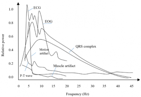
The frequencies of components participating in the ECG recording signal include muscle artifacts (5 – 50 Hz), respiratory artifacts (0.12 – 0.5 Hz), electrooculogram (EOG) artifacts (0.1 – 20 Hz, corresponding to 8 – 30 bpm), power line artifacts (50 or 60 Hz), and other electrical sources, typically greater than 10 Hz (e.g., muscle stimulators, strong magnetic fields, and pacemakers with impedance monitoring) [3, 4]. The electrode-skin interface warrants particular attention as it constitutes the most significant source of interference, producing a DC component of approximately 200-300 mV [5, 6]. Comparing the noise amplitude with the patient's heart electrical activity (typically between 0.1 and 2 mV) reveals that noise from this component is amplified through body movements or changes in the patient's position or respiration [7]. The relative amplitude-frequency graph of the QRS complex, P-T wave, muscle artifacts, motion artifacts, and ECG signal's frequency distribution is depicted in Figure 1.
Relative power spectra of QRS complex, P and T wave, muscle and motion artifacts based on an average value of 150 heart beats.
Normally, the interference filtering system on the ECG recording signal is performed 4 times: high-pass filtering, low-pass filtering, notch filtering and common mode filter. High pass filter to remove low frequency signals (i.e., only higher frequencies can pass) and low pass filter to remove high frequency signals.
Out of the basic interference components as described above, the ECG recording signal also exhibits many other abnormal patterns, those are samples that have a sudden change in amplitude and frequency due to the impact from unwanted ingredients [8]. Furthermore, each electrode is also affected by other biomedical signal components during signal acquisition, such as electromyogram, electroencephalogram, and Electrooculogram..., especially the motion artifacts that occurs with voluntary or involuntary patient movement during ECG recording.
Figure 1. Amplitude-frequency distribution graph in ECG recording signal
Many studies have focused on eliminating artifact on ECG recording signals with different approaches such as Motion artifact removal (MR); QRS detection based Motion Artifact Removal algorithm (QRSMR) [9]; Stationary Wavelet Movement Artifact Reduction (SWMAR); Normalized Least Mean Square Adaptive Filter technique (NLMSAF) [10]; moving average filtering, and wavelet transform have been used to reduce the motion ECG artefact [11, 12]; removing such ECG artifacts from local field potentials (LFPs) recorded by a sensing-enabled neurostimulato [13]; ECG Artifact Removal from Single-Channel Surface EMG Using Fully Convolutional Networks [14], Channel-Wise Average Pooling and 1D Pixel-Shuffle Denoising Autoencoder for Electrode Motion Artifact Removal in ECG [15], Removing Cardiac Artifacts From Single-Channel Respiratory Electromyograms [16].
The ECG signal recorded at the electrodes is a complex mixture of many components that come from different sources and are difficult to isolate. Using Independent Component Analysis (ICA) can help separate these sources into independent components (ICs), making it possible to remove unwanted components.
However, the accuracy of ICA is highly dependent on the size of the analytical database [16], usually the number of signal sources in the body always exceeds the number of data
recording channels; and in this case, ICA will not be able to separate the interference from the remaining components, or the components that are considered as artifacts, when removed still contain useful information, so the artifact cancellation will cause information loss.
An effective technique used in signal analysis is the wavelet transform (WT), which allows multi-resolution decompostion on different scales based on the wavelet coefficients, from which We can determine exactly the signal frequency over time. Because interference components are often concentrated on certain frequency bands, eliminating artifact on each coefficient of wavelets will be a good solution to overcome the disadvantages of ICA. In combination with ICA, WT allows ICs to continue to decompose more level on multiple scales from the coefficients of the wavelet, artifact suppression performed on every coefficient of the wavelet has enhanced the ability of the system, and it is also known as Wavelet enhanced ICA (wICA). Artifact suppression will be achieved by setting a hard threshold on each wavelet coefficient according to the formula:
$T=\sigma \sqrt{2 \log (k)}$ (1)
with $\sigma^2=\operatorname{median}\left(\left|a_{i j}\right|\right) / c$ .
For (aij) are the wavelet coefficients, k is the length of the data segment to be processed and c is a constant [15].
wICA is widely applied in recent years based on its advantages; however, the wICA tool still has limitations when it comes to noise components that change dramatically in amplitude, then changing the threshold value based on changing the mean value (aij) is not enough to remove this artifact componence. As such, flexible threshold values are needed in order to obtain optimal ECG signals at the output. From analysis of the above, a new solution was proposed, that is a combination of wICA and adaptive filters (wICAAF) is developed in this research. Based on this new way, threshold T will continuously update at the time t, t+1, t+2 ... after each input epoch, so the threshold values would be adjusted adaptively to suit the appearance of artifacts. The wICAAF solution has shown superior experimental results in removing artifacts from ECG recordings compared to the previous method; The correlation coefficient of the signal after noise cancellation compared to the reference signal of the new solution has reached 0.9832 compared to the coefficient of 0.9690 of the wICA system.
2.1 Experimental database
Experiments in the study used ECG data from PhysioBank Database, which's available at www.physionet.org. ECG recordings were selected randomly from 25 patients (10 females and 15 males) of the 92-person dataset in the data bank; all subjects had a history of cardiovascular disease. Each subject's data was recorded on traditional ECG signal channels, which included nine true unipolar leads: three limb potentials (LA, RA, LL) and six unipolar precordial leads (UV1: UV6); the sampling frequency of the signal is 800Hz. The Data is preprocessed through a bandpass filter with a cutoff frequency from 0.5 to 150Hz before being used in artifact suppression experiments. Each subject was allowed to use 02 data records; one raw data used for experiments and 01 clean data system (removed interference components) used as a reference base to evaluate the system's artifact suppression ability.
Each record is segmented into 10-second data segments (an epoch). Since the duration of data recorded on each subject in the data bank is different, the author selected 40 random signal epochs on consecutively each subject; thus, the total number of data participating in the experiment is 1000 epochs (10-second segments). The subjects participating in the experiment were between 20 and 60 years old with an average age of 42.88 years; all of whom are being treated in the hospital.
2.2 ICA and interference suppression operation
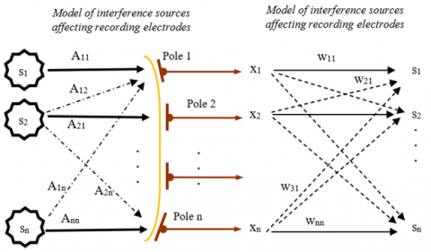
The operation of the ICA is based on factors such as: the analytical data must be a stable combination of biomedical signals and other interference sources; the recording signals originate from different sources on the body and are linear at the electrodes, the delay time of the signal from the source to the electrodes is negligible; the number of signal sources should not exceed the number of electrodes too much [15, 17]. From here, the analysis of the ICA method will be based on the principle as shown in the Figure 2.
Figure 2. The recording signal is a combination of different sources at the electrodes and the ICA's separation of sources
For s1, s2, …, sn: different signal sources; electtrodes 1~ n: electrodes that record the received signals; x1, x2, …, xn: the recording signals; Aij: signal mixing coefficients; Wij is the coefficients of the matrix W (W: the inverse of the A matrix).
The signal recorded at the electrodes can be considered as a linear combination of signals from different sources, they must have a statistically independent and non-Gaussian distribution according to the formula x=A.s; (n signal source must correspond to n electrodes), so A will be an n x n matrix where Aij are the coefficients corresponding to the mixing of independent signals from n different sources; and so only the recording signal 'x' can be observed. With the task of ICA is to analyze the sources s, so the value of source s is calculated by the formula: s=W.x with W=A−1. However, we can't determine the value of A−1 directly because we don't really know about the coefficients 'Aij' and value of the signal emitted from the source s.
The ICA model imposes a limitation that the independent components must be non-Gaussian, it's mean that the probability density function must have non-Gausian distribution. Thus, Gaussian random variables are determined entirely by first-order statistics (mean) and quadratic statistics (variance), the higher-order statistics being zero. The ICA model needs higher order statistics of the independent components to perform the independent component estimation. Thus, nonlinearity, non-Gaussianity leads to statistical independence. Signal sources "si" need to contain the least Gaussian components, so the Non-Gaussian maximization measurement is the key to evaluating the matrix weights A or independent components.
To estimate one of the independent components, we consider a linear combination of the xi; let us denote this by y=wTx=∑wixi, where w is a vector to be determined. If w were one of the rows of the inverse of A,
To solve the problem of ICA estimation, we need to "maximize non-Gaussianity" (nongaussianity). An important parameter used to measure non-Gaussiness is negentropy, which is used to maximize non-Gaussianity, leading to the development of fast computation algorithm "FastICA". Negentropy J(Y) is used as a measure of Non-Gaussian Maximization, which is an information theory-based quantity called differential entropy.
$J(Y)=H\left(Y_{g a u s s}\right)-H(Y)$ (2)
For Y is a random variable, H(Ygauss) is the entropy value of a Gaussian variable which correspond to Y matrix.
An approximation method has been developed:
$J(y)=\left\{E[G(Y)]-E\left[G\left(Y_{\text {gculss }}\right)\right]\right\}^2$ (3)
The FastICA Algorithm:
The FastICA is based on a fixed-point iteration scheme for finding a maximum of the nongaussianity of wTx, it can be also derived as an approximative Newton iteration. Denote by g the derivative of the nonquadratic function G is:
The nonlinear function G(.) can be selected according to one of the following two expressions:
$\left[\begin{array}{l}G(u)=\frac{1}{a} \log \cos a u ;(1 \leq a \leq 2) \\ G(u)=-e^{-\frac{u^2}{2}}\end{array}\right.$ (4)
g(.) is the derivative of functions G(.); corresponding to:
$\left[\begin{array}{l}g(u)=\tanh (a u) \\ g(u)=u e^{-\frac{u^2}{2}}\end{array}\right.$ (5)
where, 1≤a≤2 is some suitable constant, often taken as a=1. The basic form of the FastICA algorithm is as follows:
1. Choose an initial weight vector w
2. Let $w^{+}=E\left\{x g\left(w^T x\right)\right\}-\mathrm{E}\left\{g^{\prime}\left(w^T x\right)\right\} \mathrm{w}$
3. Let $w=w^{+} /\left\|w^{+}\right\|$
4. If not converged, go back to 2
The one-unit algorithm of the preceding subsection estimates just one of the independent components, or one projection pursuit direction. To estimate several independent components, we need to run the one-unit FastICA algorithm using several units (e.g., neurons) with weight vectors w1, w2, ..., wn.
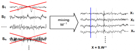
With matrix W (vectors w1, w2, ..., wn), we can separate n independent components, the next job is to evaluate which independent components are unwanted components to remove. The interference cancellation is the setting of 0 values for the unwanted components, so after recombining the independent components (ICA inverse), we will get a clean signal. The model of interference cancellation by ICA is shown in Figure 3.
Figure 3. Interference suppression model based on the ICA method
2.3 Model of combining ICA and wavelet transform in artifact suppression
As analyzed above, the operation of the ICA is based on the analysis of independent sources; next step, the artifact suppression work will be removing the analyzed independent components (ICs) that are evaluated as interference. However, if the removed independent component still contains useful information (signal components originating from the patient's heart), this may result in a loss of information useful for clinical diagnosis. To overcome this problem, the solution is to perform artifact suppression only in certain frequency ranges. Thus, each independent component will be decomposed into sub-bands. The subband analysis will be based on the spectrum of the important and prominent components in the ECG recording signal.
2.3.1 Spectral range of the main components in the received signal
There are many components in the ECG recording signal, their frequency distribution will depend on different pathological states. However, the power spectrum of the ECG's principal component is in the ranges of 1 ~ 20 Hz, signal amplitude will decrease as frequency increases and quickly disappear in the frequency range above 12 Hz; thus, the frequency component from 1 to 12 Hz will be selected to recognize as many ECG rhythms as possible. These spectra are not affected by high frequency components above 20 Hz such as power line interference (50/60 Hz), some forms of muscle artifacts; and are also not affected by interference of very low frequency components (<0.5 Hz) such as baseline drift and respiratory [18, 19]. Heart rate and P waves appear in the frequency range of 0.67~5 Hz, T waves in the frequency range 1~7 Hz, QRS components in the frequency range: 10-50 Hz. therefore, the muscle artifact component (EMG), Electrooculogram artifacts (EOG) are in the frequency range of 5~50Hz is the factors that greatly affects the ECG recording signal. In addition, there are many other components involved in the recording signal (the components that their frequencies>10Hz) such as muscle stimulator, strong magnetic field interference, pacemaker with impedance monitoring etc. also have also significantly affect the amplitude - frequency of the ECG signal. Through the above analysis, we will decompose each ICs into some subbands to conveniently remove artifacts and unwanted effects.
2.3.2 Subband decomposition using Discrete Wavelet Transform
There are different methods to decompose a signal into several subbands; with traditional methods, the researchers often apply the short time Fourier transform (STFT), this method use a window function during so short time enough that the signal segment is considered as stationary signal, then Fourier transform will perform frequency analysis; thus, it is considered that we have located the signal frequency over time.
However, the size of the window is a problem posed; because in order to achieve high accuracy when analyzing frequency components, the window size must vary flexibly according to the occurrence of each frequency.
To solve this windowing problem, wavelet transform is used to overcome the limitation of fourier transform. Wavelet transform allows flexible use of 'windows’ sizes according to multi-resolution analysis; the large 'windows' for low frequency signals; and short windows, and small 'window' for high frequency signals. In other words, it adjusts the size of the window to accommodate every frequency [20, 21].
x[n] is input signal, g[n] is the high-pass filter, h[n] is the low-pass filter, and C is coefficient matrix which is decomposition of wavelet coefficients
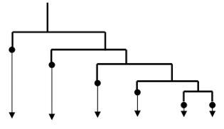
The Discrete Wavelet Transform (DWT) uses filter banks to create the multiresolution time-frequency domain, they're special wavelet filters for the decomposition and reconstruction of signals; Sub-band decomposition of Discrete Wavelet Transform (DWT) is implemented as the Figure 4.
Figure 4. DWT decomposition
The outputs of high-pass filter give the detail coefficients and low-pass filter give approximation coefficients (two filters are related to each other and called as a quadrature mirror filter). Because half the frequencies of the signal have now been removed, half the samples can be discarded according to Nyquist’s rule. The filter output of the filter is then subsampled by 2
Figure 5. Discrete Wavelet Transform at level 5 and obtained subbands
With the pre-processing ECG frequency in the range 0.5 to 150Hz, discrete wavelet decomposition will be performed at level 5; thus, subband analysis can obtain wavelet coefficients (aij) corresponding to the important bands of the ECG signal, such as T-wave, P-wave, QRS complex, and isolate some interference components etc., in order to eliminate the artifact concentrated in each area, increasing the system's efficiency. The decomposition diagram in the level 5 with obtained subband is shown in Figure 5.
Table 1. The wavelet coefficients
|
No. |
Wavelet coefficients |
Frequency ranges |
|
1 |
Band a1 |
0.5~4.7Hz |
|
2 |
Band a2 |
4.7 ~9.4Hz |
|
3 |
Band a3 |
9.4~18.8 Hz |
|
4 |
Band a4 |
18.8~37.5 Hz |
|
5 |
Band a5 |
37.5~75Hz |
|
6 |
Band a6 |
75~150Hz |
Thus, the input signal 'ECG' passes through the ICA system and is analyzed into independent components; these components will be further decomposed into wavelet coefficients (aij) in Table 1; the soft threshold values will be set on each coefficient (aij).
The threshold value is calculated according to the formula:
$T=\sigma \sqrt{2 \log (k)}$ (6)
for k is the length of the analyzed data segment and σ is defined as:
$\sigma^2=\frac{\operatorname{mean}\left(\left|a_{\mathrm{ij}}\right|\right)}{c}$ (7)
with c is set to 0.858.
With a sampling frequency of 800Hz, the value of k is set to 8000 (an epoch);
$T=\sigma \sqrt{2 \log (k)} \sim 2.79 \sigma$ (8)
Thus, it is easy to see that the threshold T will change corresponding to the value of the coefficients aij.
The artifact removal algorithm with the threshold solution T is as follows:
$\hat{a}_{i j}= \begin{cases}\operatorname{sign}\left(a_{i j}\right)\left(\left|a_{i j}\right|-T\right) & \text { if }\left|a_{i j}\right|>T \\ a_{i j} & \text { if }\left|a_{i j}\right|<T\end{cases}$ (9)
After removing artifact components on the wavelet coefficients, the next step will be the inverse wavelet transform (IWT) to obtain the clean IC components; at the end, the inverse ICA transform will give us a clean signal 'ECG' with artifact components removed. This model has overcome some inherent limitations of ICA as analyzed above, so it is also known as wavelet enhanced ICA or wICA.
2.4 Model of combining wICA and adaptive filter in artifact suppression
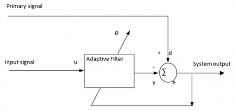
Adaptive filter: The ability of an adaptive filter to work effectively in an unknown or constantly fluctuating environment and track time variations of input statistics makes the adaptive filter a powerful device for signal processing and control application.
Adaptive filters have been successfully applied in fields as diverse as communications, radar or biomedical engineering. Although the applications are quite different in nature, but they have one basic common feature: An input vector and a desired response are used to calculate the estimation error (which used to control the values of a set of adjustable filter coefficients) [22, 23]. The adjustable coefficients can be in the many different forms depending on the filter construction used. However, the fundamental difference between different applications of adaptive filtering arises in the manner in which the desired response is extracted. In the requirement to eliminate the artifact of the ECG signal, the adaptive filter model applied in interference suppression as shown in Figure 6 is used; this model will be coordinated with the wICA system to improve the artifact suppression efficiency.
Figure 6. Adaptive filter model - the type of interference cancellation
y=output of the adaptive filter.
d=desired response.
u=input signal applied to the adaptive filter.
The estimation error:
$e=d-y$ (10)
In this model, the primary signal serves as the desired response for the adaptive filter; a reference signal is employed as the input to the filter; the reference signal is derived from a sensor or a set of sensors located such that it supplies the primary signal in a way that the information-bearing signal component is weak or essentially undetectable [22].
2.5 Combination of wICA and adaptive filtering model
Although ICA is able to detect and remove interlaced components not originating from the patient's heart, however they are often suspected to remove some of the useful signals from the myocardium. To solve this problem, wavelet decomposition is applied to analyze each independent component (IC) into smaller components; The generated noise removal is performed on each coefficient of the wavelet (aij) to obtain clean ICs without information loss. However, the survey results show that the effectiveness of the generated interference cancellation will be reduced when appearing some artifacts with the amplitude of continuous change in a narrow range; the reason is caused by the flexibility of the threshold value that has not kept up with the rapid & continuous changes in the amplitude of the artifact.
From (6), it is easy to see that the threshold value (T) is related to both parameters, that is the average amplitude value of the wavelet coefficients (aij) and the length of the data segment (k), but the change of segment 'k' does not have much effect on the threshold value (T); the parameter that mainly affects the T value is aij's amplitude (If aij's components that are mainly artifacts, then the change of the average artifact amplitude will be main factor to changes T value significantly). Because as explained above, $T=\sigma \sqrt{2 \log (k)} \sim 2.79 \sigma$ and $\sigma^2=\frac{\operatorname{mean}\left(\left|a_{\mathrm{ij}}\right|\right)}{c}$, so the threshold level will be closely related to the average energy of the signal. Thus, in some cases, when the ECG recording signal is contaminated with many artifact components with rapidly and continuously varying amplitudes in a narrow range, the soft threshold level (T) will change suddenly, causing signal distortion after noise cancellation; in other words the threshold will not be flexible enough to eliminate the artifacts effectively.
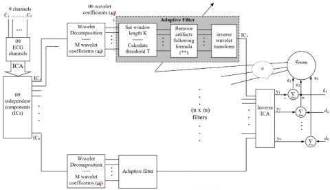
The proposed model is as shown in Figure 7.
Figure 7. Model of combining wICA and adaptive filter in artifact suppression (wICAAF)
Based on the wICAAF model, the threshold values 'T values' will be adjusted to suit the variation of the artifact. The desired response inputs (d1~d9) are applied to evaluate the estimation errors (e) of the output signal from the system (after denoising); e value is the basic parameter used to adjust the threshold T according to the principle: the next T value tends to reduce 'e value' to zero.
The threshold level T will limit the amplitude values on each wavelet coefficients (aij) according to the formula (**); where e1, …, e9 are estimation errors of 9 channels and calculated by difference of (di–yi); emean: the mean of estimation errors on 9 channels, C1, …, C9: ECG channels, y1….y9: 09 channels after denoising, d1, …, d9: desired response for 9 ECG channels; m is the number of wavelet coefficient (in our study, m=6)
'Estimation error - e' is calculated by the mean of the error function over the output channels:
$e=\operatorname{mean}\left(e_i\right)=\frac{\sum_i\left(e_i\right)}{n}$ for $i\{1 \ldots n\}$ with $n=9$ (11)
The estimation error ei will be applied to each adaptive filter on the system, and the adaptive filters is considered as nominal filters. The value of e also can be used to evaluate the efficiency of the whole system in the case of combining and uncombing with adaptive filtering model.
From the wICA system, the research team has developed an algorithm for the wICAAF system, the method of removing artifacts on the wavelet coefficient is implemented according to the formula below.
$\hat{a}_{i j}(t)=\left\{\begin{array}{l}\operatorname{sign}\left[a_{i j}(t)\right]\left[\left|a_{i j}(t)\right|-T_{i j}(t)\right] \text { if }\left|a_{i j}(t)\right|>T_{i j}(t) \\ a_{i j}(t) \text { if }\left|a_{i j}(t)\right|<T_{i j}(t)\end{array}\right.$ (12)
With $\hat{a}_{i j}(t)$ are the signal components after removing the artifacts at time t; aij(t) are wavelet coefficients at time t for i{1…9) and j{1…m}, in our study m=6; Tij(t) is the threshold level at time t in the ith independent component, the jth wavelet coefficient.
Because there are some types of artifact, which converge on only a few bands, but their amplitude varies rapidly and continuously, thereby reducing the ability of the system to eliminate artifacts; this is also the main cause of the estimation error (ei) or the deviation between the output signal and the desired response. With wavelet coefficients that wasn't affected by artifacts, aij's amplitude value would be relatively stable; the estimated error (ei) would be close to zero. With the above analysis, we set up the formula for threshold T:
Following formula (8),
$T=\sigma \sqrt{2 \log (k)} \sim 2,79 \sigma ; \sigma^2=\frac{\operatorname{mean}\left(\left|a_{j k}\right|\right)}{c}$
$\sigma_{t+1}=\sqrt{\frac{\operatorname{meab}\left(\left|a_{i j}\right|\right)_{t+1}+e_t}{c}}$ (13)
$T_{t+1}=\sigma_{t+1} \sqrt{2 \log k}$ (14)
For et is the mean of the estimation error at time t, $\operatorname{mean}\left(\left|a_{i j}\right|\right)_{t+1}$ is the mean absolute value of the wavelet coefficients at time (t+1) and $T_{t+1}$ is a threshold value at time (t+1); ei=mean(di)–mean(yi).
With some ICs that was not affected by artifacts at time t, the estimation error at time t (et) will correspond to zero; so at time t+1, the threshold value T would have no the correction. Thus, the threshold value is only corrected at the time of the impact of the anomalous artifact.
Advantage: methods using soft threshold T in artifact suppression for better signal quality, especially they retain detailed and useful information of cardiac activity to support diagnostic jobs for pathological phenomenons.
Disadvantage: The artifact removal is also approximate; moreover, this adaptive threshold value would be changed only when the impact of the artifact caused appearing the estimation error value at the output. Thus, the change in threshold values wasn't really timely and optimal.
Experimental data from the data bank, available at www.physionet.org were obtained from 25 subjects participating in our experiment, evaluation data were selected 40 random signal segments on consecutively each subject. The database system on each subject is segmented into epochs, a 10-second data segment with a sampling rate of 800Hz, the subjects participating in the experiment all had a history of heart disease, and are currently being monitored and treated at Campbelltown hospital - Australia [24].
Before using the data in the artifact suppression and evaluation experiments, the data is preprocessed through a bandpass filter with a cutoff frequency from 0.5 ~ 150Hz to remove some basic noise which are out-of-band frequency of the useful signal components, so that the system can mainly focus on eliminating the complex interference components that mix in the recorded signal.
A correlation coefficient is a numerical measure of some type of correlation, meaning a statistical relationship between two variables. In our study, the correlation value will be used to evaluate the correspondence of the signal after artifact suppression and the reference signal.
Some clean epochs were extracted manually by technical experts on the total of 09 channels for every subject what were used as desired response of the adaptive filter system. The effectiveness of the artifact suppression process will be analyzed and evaluated based on the correlation coefficient R between the output signal of the wICAAF system and the reference signal (Rmax=1). The window width k is set to 800 corresponding to 01 second of data and the wavelet function used is Daubechies.
The effectiveness of the new artifact suppression method will be evaluated based on the comparison of the wICAAF system with previous methods such as ICA, wICA. The correlation coefficient between the signal after denoising and the reference signal (desired response) of all three methods ICA, wICA, wICAAF is performed on all 9 channels as described in Table 2.
Table 2. The comparison table of r value in artifact removal between wICA & wICAAF method
|
No |
Unipolar leads |
R value |
||
|
ICA |
wICA |
wICAAF |
||
|
1 |
I |
0.9195 |
0.9595 |
0.9708 |
|
2 |
II |
0.9266 |
0.9636 |
0.9786 |
|
3 |
III |
0.9182 |
0.9762 |
0.9818 |
|
4 |
V1 |
0.9249 |
0.9549 |
0.9841 |
|
5 |
V2 |
0.931 |
0.9697 |
0.9933 |
|
6 |
V3 |
0.9208 |
0.9796 |
0.9855 |
|
7 |
V4 |
0.9038 |
0.9812 |
0.9817 |
|
8 |
V5 |
0.9105 |
0.9573 |
0.9796 |
|
9 |
V6 |
0.9094 |
0.9794 |
0.9934 |
|
|
Mean |
0.9183 |
0.9690 |
0.9832 |
The correlation coefficients were calculated by $R=\frac{C_{x y}}{\sigma_x \sigma_y}$ ($C_{x y}$ is the co-variance of $x$ and $y$, and $R \leq 1$) for $C_{x y}=$ $E\left\{\left(x-\eta_x\right)\left(y-\eta_y\right)\right\}, \quad E\{x\}=\eta_x, E\{y\}=\eta_y, \quad \sigma_x=$ $\sqrt{E\left\{\left(x-\eta_x\right)^2\right\}}$ and $\sigma_y=\sqrt{E\left\{\left(y-\eta_y\right)^2\right\}}$ [25].
With x is the reference signal (which is manually cleaned by experts and used as a desired response); y is the signal after going through the wICAAF system; $\vdots \eta_x=\bar{x}$ {the mean of x(i)}; $\eta_y=\bar{y}$ {the mean of y(i)}; $C_{x y}=E\left\{\left(x-\eta_x\right)\left(y-\eta_y\right)\right\}$ is caculate by the fomular $C_{x y}=\operatorname{Cov}(x, y)=\frac{\sum(x-\bar{x})((y-\bar{y})}{n-1}$ and $\sigma_x^2=\frac{\sum(x-\bar{x})^2}{n-1} ; \sigma_y^2=\frac{\sum(y-\bar{y})^2}{n-1}$ with (n-1) is the number of samples in each epoch that removed artifact.
The correlation coefficient will evaluate the similarity between the signal after noise suppression and the desired response; As a result, the mean value of the correlation coefficient on a total of 09 channels showed that the quality of artifact cancellation of the wICAAF system was improved significantly since the R mean value reached 0.9832, while the R value of the system ICA system only achieved 0.9183 and wICA system also achieved 0.9690.
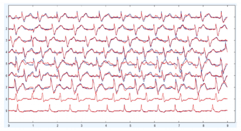
The green line below is the signal after denoising by wICA and the red line above is the signal after going through the wICAAF system.
Completely removing unwanted independent components (ICs) can cause information loss, however setting a threshold level with low flexibility as described in the wICA method can still cause useful information loss from the recording signal. The adaptive thresholding solution on wavelet coefficients has shown positive results compared to the traditional method, both improving the artifact suppression of the system and allowing to reduce distortion of the recorded signal as showed on Figure 8.
Figure 8. Artifact suppression and signal distortion by the wICA and wICA combined adaptive filter (wICAAF) model
In this study, the author has proposed the wICAAF model, a solution that combines wICA with adaptive filtering in artifact suppression, the proposed model has overcome the inherent limitation of wICA that is reduced efficiency when appearing abnormal artifact components, rapidly changing in both amplitude and frequency, especially EMG components. The proposed method has proved to have many advantages over the previously used methods based on the positive data of experimental results. This interference cancellation model can be effectively applied to the artifact cancellation of the ECG signal in particular, or the biomedical signal in general; It is also effective in applying interference suppression to acquiring the data on the multi - channels system similarly.
However, the processing data are only taken from the biomedical data bank to apply in our experiments, many specific pathological states of cardiovascular problems have not been mentioned. In fact, there are many different cardiovascular conditions that greatly influence the recording of ECG signals. So a more comprehensive assessment will be the task of research team in the future; the number of participants and the epoch number on each subject also increasing significantly in the next author's experiments.
The author gratefully acknowledges the University of Economics – Technology for Industries for supporting this work.
[1] Lanata, A., Guidi, A., Baragli, P., Valenza, G., Scilingo, E.P. (2015). A novel algorithm for movement artifact removal in ECG signals acquired from wearable systems applied to horses. PloS One, 10(10): e0140783. https://doi.org/10.1371/journal.pone.0140783
[2] Elgendi, M., Meo, M., Abbott, D. (2016). A proof-of-concept study: Simple and effective detection of P and T waves in arrhythmic ECG signals. Bioengineering, 3(4): 26. https://doi.org/10.3390/bioengineering3040026
[3] Raheja, N., Manocha, A.K. (2020). Removal of Artifcats in Electrocardiograms using Savitzky-Golay Filter: An Improved Approach. Journal of Information Technology Management, 12: 62-75. https://doi.org/10.22059/jitm.2020.78890
[4] Phadikar, S., Sinha, N., Ghosh, R., Ghaderpour, E. (2022). Automatic muscle artifacts identification and removal from single-channel EEG using wavelet transform with meta-heuristically optimized non-local means filter. Sensors, 22: 2948. https://doi.org/10.3390/s22082948
[5] Sedaghat, G., Gardner, R.T., Kabir, M.M., Ghafoori, E., Habecker, B.A., Tereshchenko, L.G. (2017). Correlation between the high-frequency content of the QRS on murine surface electrocardiogram and the sympathetic nerves density in left ventricle after myocardial infarction: Experimental study. Journal of electrocardiology, 50(3): 323-331. https://doi.org/10.1016/j.jelectrocard.2017.01.014
[6] Babusiak, B., Borik, S., Smondrk, M. (2020). Two-electrode ECG for ambulatory monitoring with minimal hardware complexity. Sensors, 20(8): 2386. https://doi.org/10.3390/s20082386
[7] Noto, B., Roll, W., Zinken, L., et al. (2022). Respiratory motion correction in F-18-FDG PET/CT impacts lymph node assessment in lung cancer patients. EJNMMI Research, 12(1): 61. https://doi.org/10.1186/s13550-022-00926-7
[8] Kher, R. (2019). Signal processing techniques for removing noise from ECG signals. Journal of Biomedical Engineering and Research, 3: 101.
[9] Zou, C., Qin, Y., Sun, C., Li, W., Chen, W. (2017). Motion artifact removal based on periodical property for ECG monitoring with wearable systems. Pervasive and Mobile Computing, 40: 267-278. https://doi.org/10.1016/j.pmcj.2017.06.026
[10] Taha, L., Abdel-Raheem, E. (2020). A null space-based blind source separation for fetal electrocardiogram signals. Sensors, 20(12): 3536. https://doi.org/10.3390/s20123536
[11] Ziani, S., Jbari, A., Bellarbi, L., Farhaoui, Y. (2018). Blind maternal-fetal ECG separation based on the time-scale image TSI and SVD-ICA methods. Procedia Computer Science, 134: 322-327. https://doi.org/10.1016/j.procs.2018.07.179
[12] Ding, J., Tang, Y., Chang, R., Li, Y., Zhang, L., Yan, F. (2023). Reduction in the motion artifacts in noncontact ECG measurements using a novel designed electrode structure. Sensors, 23(2): 956. https://doi.org/10.3390/s23020956
[13] Chen, Y., Ma, B., Hao, H., Li, L. (2021). Removal of electrocardiogram artifacts from local field potentials recorded by sensing-enabled neurostimulator. Frontiers in Neuroscience, 15: 637274. https://doi.org/10.3389/fnins.2021.637274
[14] Wang, K.C., Liu, K.C., Peng, S.Y., Tsao, Y. (2023). ECG Artifact removal from single-channel surface EMG using fully convolutional networks. In ICASSP 2023-2023 IEEE International Conference on Acoustics, Speech and Signal Processing (ICASSP), Rhodes Island, Greece, pp. 1-5. https://doi.org/10.1109/ICASSP49357.2023.10096409
[15] Chiu, C.C., Hai, B.H., Yeh, S.J., Liao, K.Y.K. (2014). Recovering EEG signals: Muscle artifact suppression using wavelet-enhanced, independent component analysis integrated with adaptive filter. Biomedical Engineering: Applications, Basis and Communications, 26(5): 1450063. https://doi.org/10.4015/S101623721450063X
[16] Petersen, E., Sauer, J., Graßhoff, J., Rostalski, P. (2020). Removing cardiac artifacts from single-channel respiratory electromyograms. IEEE Access, 8: 30905-30917. https://doi.org/10.1109/ACCESS.2020.2972731
[17] Martinek, R., Kahankova, R., Jezewski, J., et al. (2018). Comparative effectiveness of ICA and PCA in extraction of fetal ECG from abdominal signals: Toward non-invasive fetal monitoring. Frontiers in Physiology, 9: 648. https://doi.org/10.3389/fphys.2018.00648
[18] Bui Huy, H. (2021). The artifact removal from ECG recording based on wavelet coefficients on independent components of ICA. Journal of Military Science and Technology, (74): 44-51.
[19] Kahl, L., Hofmann, U.G. (2021). Removal of ECG artifacts affects respiratory muscle fatigue detection - A simulation study. Sensors, 21(16): 5663. https://doi.org/10.3390/s21165663
[20] Hesar, H.D., Mohebbi, M. (2015). Muscle artifact cancellation in ECG signal using a dynamical model and particle filter. In 2015 22nd Iranian Conference on Biomedical Engineering (ICBME), Tehran, Iran, pp. 178-183. https://doi.org/10.1109/ICBME.2015.7404138
[21] Lin, C.C., Chang, H.Y., Huang, Y.H., Yeh, C.Y. (2019). A novel wavelet-based algorithm for detection of QRS complex. Applied Sciences, 9(10): 2142. https://doi.org/10.3390/app9102142
[22] Gualsaquí, M., Vizcaíno, I., Rosero, V.G.P., Calero, M.J.F. (2018). ECG signal denoising using Discrete Wavelet Transform: A comparative analysis of threshold values and functions. Maskana, 9(1): 105-114. https://doi.org/10.18537/mskn.09.01.10
[23] Shaddeli, R., Yazdanjue, N., Ebadollahi, S., Saberi, M. M., Gill, B. (2021). Noise removal from ECG signals by adaptive filter based on variable step size LMS using evolutionary algorithms. In 2021 IEEE Canadian Conference on Electrical and Computer Engineering (CCECE), ON, Canada, pp. 1-7. https://doi.org/10.1109/CCECE53047.2021.9569149
[24] Lakhera, N., Verma, A.R., Patel, S.S., Gupta, B. (2021). A novel approach of ECG signal enhancement using adaptive filter based on whale optimization algorithm. Biomedical and Pharmacology Journal, 14(4): 1895-1903. https://dx.doi.org/10.13005/bpj/2288
[25] Gargiulo, G.D., McEwan, A.L., Bifulco, P., Cesarelli, M., Jin, C., Tapson, J., Thiagalingam, A., Van Schaik, A. (2013). Towards true unipolar ECG recording without the Wilson central terminal (preliminary results). Physiological Measurement, 34(9): 991. https://doi.org/10.1088/0967-3334/34/9/991