Marwah Abdullah Shlash*![]() | Imad Habeeb Obead
| Imad Habeeb Obead![]()
© 2023 IIETA. This article is published by IIETA and is licensed under the CC BY 4.0 license (http://creativecommons.org/licenses/by/4.0/).
OPEN ACCESS
Addressing the global water depletion challenge, this study integrates five supervised machine learning algorithms (MLAs) with GIS-based techniques to assess groundwater potential. The employed MLAs include Ensemble Boosted Trees (logic-based learners), Naive Bayes (NB; statistical learning algorithms), Support Vector Machines (SVM), Multi-Layer Perceptron (MLP; Artificial Neural Networks), and k-Nearest Neighbors (kNN; instance-based learners). These MLAs were utilized to generate groundwater potential maps (GPMs) based on seven influential variables: aquifer unit types, transmissivity, lineament density, slope, soil type, land use/land cover, and drainage density. Classifier performance was evaluated using metrics such as True Positive Rates (TPR), False Negative Rates (FNR), Positive Predictive Values (PPV), False Discovery Rates (FDR), and the Area Under the Curve (AUC) of Receiver Operating Characteristic (ROC) curves. Results indicate that kNN-based learners outperformed other methods, achieving a validation accuracy of 90.70% and an AUC of 1, which corresponds to 100% accurate predictions. Ensemble Boosted Trees, MLP, SVM, and NB followed, with validation accuracies of 89.7%, 79.4%, 77.6%, and 75.7%, respectively. The methodology developed in this study can be applied to estimate and manage potential groundwater resources in regions facing water scarcity issues.
machine learning, supervised classification, Artificial Neural Networks (ANN), Groundwater Potential Mapping (GPM)
Groundwater serves as a crucial resource in arid and semi-arid regions, as aquifers offer a sustainable source of high-quality water throughout the year when rainfall and surface water are scarce. Due to climate change, rainfall is anticipated to decrease, and droughts are expected to become more severe [1]. Generally, the term "groundwater potential" refers to the amount of groundwater available in an area and depends on various hydrologic and hydrogeological factors. From a hydrogeological perspective, this term can be defined as the probability of groundwater occurrence in an area or the prediction of where the highest borehole yields may be found. Proper assessment of groundwater potential can serve as a valuable guideline for decision-makers to identify appropriate groundwater strategies within an area and manage the aquifer system sustainably [2, 3].
Methods for mapping groundwater potential zones are classified into two categories: knowledge-driven techniques, such as the Analytical Hierarchy Process (AHP), which are based on expert experiences and thus influenced by specialist knowledge and subjectivity, and data-driven techniques, which involve probabilistic, statistical, and data mining approaches based on the empirical element of groundwater assessments [4-6]. Expert-based decision approaches have long been utilized, while machine learning is a comparatively newer method. A crucial difference between machine learning and expert techniques is that machine learning classification employs artificial intelligence capabilities to discover complex associations between explanatory factors that would otherwise remain unnoticed. Consequently, machine learning is well-suited for mapping complicated, spatially distributed variables such as groundwater occurrence [7]. Machine learning (ML) uses algorithms that can learn and improve themselves based on the experience they gain from collected data to produce accurate predictions [8]. ML can be divided into two categories: supervised and unsupervised algorithms. In unsupervised learning, the algorithm derives patterns from data that have not been labeled or otherwise categorized, aiming to understand the fundamental structure of the data. Since the model does not have a reference for the expected output data format, it cannot carry out any training on the model. Instead, the model investigates the structure of the data so that valuable information may be extracted from it [9]. Supervised learning algorithms are the preferred method when both input and output variables are clearly labeled. The goal is to learn patterns and correlations between variables based on prior experience (training data) and then apply that information to generate predictions on data that has not been seen or is unknown (test data). In supervised learning, two subcategories of data can be modeled: classification, in which a model aims to predict categorical or class labels, and regression, in which the models attempt to predict a continuous output. Both classification and regression are examples of predictive modeling [10]. The Groundwater Potential Mapping (GPM) literature presents several supervised classification strategies.
For instance, Ozdemir [11] employed a binary logistic regression to generate a groundwater spring potential map GPM of the Sultan Mountains in central Turkey using a logistic regression technique integrated with the Geographic Information System (GIS) environment. An area value of 0.82 was determined for the Receiver Operating Characteristic (ROC) curve model, indicating an accurate prediction of spring potential in the study region. Additionally, the existing groundwater spring test data and the created model were in close agreement. Nguyen et al. [12] utilized an advanced ensemble machine learning model (RABANN) that combines Artificial Neural Networks (ANN) with RealAdaBoost (RAB) ensemble approach to evaluate the groundwater potential of DakNong province, Vietnam. This work used twelve conditioning parameters and well-yield data to generate the training and testing datasets. The results indicate that the RAB ensemble approach improved the performance of the ANN model. With minor modifications to the input data, the ensemble-developed model could be applied to map the groundwater potential of other regions and countries to enhance water resource management.
Sarkar et al. [13] developed ensemble machine learning (EML) algorithms for groundwater potentiality mapping (GPM) in Bangladesh's Teesta River basin. These algorithms include random forests (RF) and random subspaces (RSS). The GPM was verified using the Receiver Operating Characteristics (ROC) curve. The random subspaces machine learning (RSS) model, with an AUC of 0.892, was determined to be the most accurate representation model for groundwater potentiality modeling, followed by random forests with an AUC of 0.86. The RSS model outperforms the RF mode in terms of groundwater potentiality models since a higher AUC indicates more accurate predictions of the model's output.
Phong et al. [14] proposed three unique ML hybrid models: modified RealAdaBoost (MRAB-FT), bagging (BA-FT), and rotation forest (RF-FT). All models are functional tree (FT) base classifiers capable of handling binary and multi-class target variables for GPM modeling in the DakLak region of Vietnam. This study employed a threshold value greater than 2 L/s for selecting training and testing datasets for groundwater classification as groundwater and non-groundwater. Standard statistical methods assessed how well the created models performed (PPV, NPV, SST, SPC, Kappa, RMSE, and ROC). The analysis' findings demonstrated that all of the unique hybrid models that had been created had high predictive abilities, but the model MRAB-FT performed the best in terms of recognizing groundwater potential zones.
Tamiru et al. [15] assessed the effectiveness of artificial intelligence (AI) in the Fincha catchment, Abay, Ethiopia, using geospatial analysis and GIS platforms to prospect possible groundwater zones. In this work, a Multi-Layer Perceptron (MLP) structure was used. The analysis' findings demonstrated that the AI models agreed with 96% of the identified groundwater potential zones and ground-truthing points, while the accuracy of the GIS platform model using the AHP method was 91%. Finally, it is stated that the ANN model is a valuable tool for defining potential groundwater zones where the cost of direct field investigation is not affordable.
Consequently, the main objective of the present study is to construct a novel hybrid model for groundwater potentiality mapping (GPM) using the performance of supervised machine learning (ML)-based techniques integrated with knowledge-driven technologies using an analytical hierarchy process (AHP) to evaluate the groundwater potential zones of Dammam confined aquifer that extended along the Najaf-Muthanna governorates using supervised learning classification.
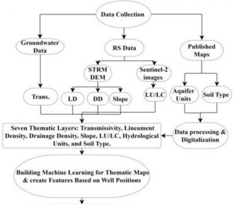
In the following sections, tools and technologies that have been used during the study will be described. Seven influencing factors on confined aquifers were considered; multi-influencing factor-knowledge-driven techniques (i.e., AHP method) were used to analyze their thematic maps using normalized weights. The developed thematic maps of influencing factors were then employed as input variables when training the ML models. The developed hybrid model can predict groundwater potentiality by analyzing the dynamic relationship between groundwater potentiality and influencing factors. The flowchart used in the current study is shown in Figure 1.
Figure 1. Methodology for supervised ML classification
It is probably reasonable to say that this study was the first to reveal the implementation of a novel hybrid-supervised classification model by applying five machine algorithms (MLAs) in Iraq: Ensemble Boosted Trees-logic-based learners, Naive Bayes (NB)-statistical learning algorithms, Support Vector Machines (SVM), Multi-Layer Perceptron (MLP)-Artificial Neural Networks (ANN), and k-Nearest Neighbours (kNN)-instance-based learners to construct GPM that contribute in the development of strategies for the sustainable management of water resources.
2.1 Study area
The study area of about 76732.71Km2 is located in Najaf and Muthanna governorates in the southern desert of Iraq. The geographic coordinates for the study area are between longitudes 44° 19 '07.68" to 46° 33' 26.55" East and between latitudes 29° 06 '15.74" to 32° 19 '55.97" North. The layout and topographic map for the study area is prepared using ArcGIS 10.7.1, as shown in Figure 2. The ground surface in the southern desert gradually increases from the southwest to the northeast by about 50m every 10-15km. The elevation of the surface increases from the Euphrates River in the east towards the south and southwest. The middle part is almost flat with many depressions [16]. The distribution and development of groundwater are primarily influenced by the various geologic formations and topographic features in which it occurs [17].
Figure 2. Maps of the study area: (a) layout map; (b) topographic map
2.2 Groundwater effective factors preparation
A range of field, documented, and remotely sensed data were collected from different government agencies to map suitable availability areas of groundwater. Seven parameters affecting the confined aquifers were considered: aquifer unit types, transmissivity, lineaments density, slope, soils, land use and land cover, and drainage density. Knowledge-driven technologies using the analytical hierarchy process (AHP) method were used to analyze their thematic maps using normalized weights to evaluate the potential groundwater zones.
The hydrogeological units' thematic map was derived based on available data and a map of the main groundwater aquifers in Iraq using the spatial analysis tools in ArcGIS 10.7.1. There are four main types of aquifer units in the study area due to different geological formations. The highest static groundwater level is recorded in the SW part of the study area, while a low groundwater level categorizes in the NE part. The general groundwater flow direction is from the elevated area at SW of the studied area toward the lower elevation to the NE [18]. The hydrogeological units of the highest static water level had the highest rank, while the aquifer units of the lowest static water level were assigned the lowest rank. The Karstified Palaeogene aquifer represents Tayarat and Dammam aquifer with good availability groundwater, the Mio-Pliocene Sandstone/Dibdiba aquifer with moderate groundwater availability, Miocene Carbonate-Ghar/Euphrates and Zahra formation with poor groundwater availability, and finally Mesopotamia Plain Silt with very poor groundwater availability. Kriging interpolation was used to generate the spatial distribution map of transmissivity; the study area was classified into five classes since it exerts substantial control on drainage density, where high transmissivity results in low drainage density and vice versa [19]. In addition, the DEM of the SRTM type, with a resolution of 30 meters, was used in creating lineament density, slope, and drainage density thematic maps utilizing spatial analysis tools included in ArcGIS 10.7.1.
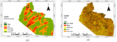
The lineament density plays a significant role in groundwater availability and movement since it noticeably exists in the study area based on the tectonic map of Iraq. Generally, the lineament density of the studied area has ranged from less than 0.022km/Km2 to 0.19km/Km2. On the other hand, the study area is classified into five classes depending on the slope variety. The areas with flat topography and slope of (0.1-0.3)ᵒ considered advantageous for groundwater recharge since the movement of runoff downstream will be decreased. In contrast, higher runoff occurred at the steep sloop.
The drainage density indirectly influences the groundwater availability due to its connection with the infiltration capacity and the permeability; higher drainage density reduces the infiltration, thus increasing the runoff; higher runoff indicates less groundwater potentiality. The study area was divided into five classes, generally ranging from less than 1km/Km2 to 17.21km/Km2.
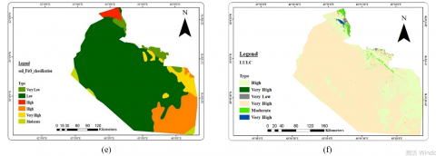
The infiltration rate also affects groundwater availability and depends on soil grain size; coarse-textured soils have a greater infiltration rate and, thus, a high groundwater potential. In contrast, medium-textured soils have moderate to poor groundwater potentiality, while fine-textured soils have the lowest infiltration rate and, thus, very poor groundwater potentiality.
Land use and land cover are essential in the area's existence and groundwater change. Consequently, the study area is divided into six classes: water, herbs wetland, herbaceous vegetation, cropland, and bare/sparse vegetation; each type has a weighted value representing the priority effect on groundwater accumulation.
In the current study, the seven thematic layers' weights were assigned for each influenced factor to generate the seven thematic maps, as shown in Figure 3.
Figure 3. Data layers for groundwater potentiality conditioning factors: (a) aquifer units; (b) transmissivity; (c) lineament density; (d) slope; (e) soil classification; (f) LULC (g) drainage density
After assigning weights to the respective parameters, individual ranks were given for sub-variables (subclasses) to calculate the final weight by multiplying each parameter's normalized weight with the rank of each sub-class in order to generate the groundwater potential zone map, as presented in Table 1.
Table 1. Weights of groundwater control parameters
|
Classes |
Normalize weight % |
Rank |
Potential index |
Final weight |
|
(1) Aquifer Units |
||||
|
Karstified Palaeogene |
38.567 |
4 |
good |
154.270 |
|
Mio-Pliocene Sandstone |
3 |
moderate |
115.702 |
|
|
Miocene Carbonate |
2 |
poor |
77.135 |
|
|
Mesopotamia Plain Silt |
1 |
very poor |
38.567 |
|
|
(2) Transmissivity (T) ( $\mathrm{m}^2$ /day) |
||||
|
9.474-12.089 |
19.284 |
1 |
very poor |
19.284 |
|
12.089-17.081 |
2 |
poor |
38.567 |
|
|
17.081-24.332 |
3 |
moderate |
57.851 |
|
|
24.332-32.414 |
4 |
good |
77.135 |
|
|
32.414-39.784 |
5 |
very good |
96.419 |
|
|
(3) Lineament Density (LD) (km/km) |
||||
|
0-0.022 |
12.856 |
1 |
very poor |
12.856 |
|
0.022-0.054 |
2 |
poor |
25.712 |
|
|
0.054-0.079 |
3 |
moderate |
38.567 |
|
|
0.079-0.114 |
4 |
good |
51.423 |
|
|
0.114-0.185 |
5 |
very good |
64.279 |
|
|
(4) Slope (SLO) (Degree) |
||||
|
0-0.1 |
9.642 |
5 |
very good |
48.209 |
|
0.1-0.2 |
4 |
good |
38.567 |
|
|
0.2-0.3 |
3 |
moderate |
28.926 |
|
|
0.3-0.5 |
2 |
poor |
19.284 |
|
|
>0.5 |
1 |
very poor |
9.642 |
|
|
(5) Soil (SL) according to FAO classification |
||||
|
Loam |
7.713 |
2 |
poor |
15.427 |
|
Loamy Sand |
3 |
moderate |
23.140 |
|
|
Sandy Loam |
4 |
good |
30.850 |
|
|
Sandy |
5 |
very good |
38.567 |
|
|
Clayey loam |
1 |
very poor |
7.713 |
|
|
(6) Land Use Land Cover (LU/LC) |
||||
|
Water |
6.428 |
5 |
very good |
32.140 |
|
Herbst wetland |
5 |
very good |
32.140 |
|
|
Herbaceous Vegetation |
4 |
good |
25.712 |
|
|
Cropland |
3 |
moderate |
19.284 |
|
|
Bare/ Sparse Vegetation |
2 |
poor |
12.850 |
|
|
Build up |
1 |
|
6.428 |
|
|
(7) Drainage Density (DD) (km/km) |
||||
|
0-1.754 |
5.510 |
5 |
very good |
27.548 |
|
1.754-4.656 |
4 |
good |
22.039 |
|
|
4.656-7.354 |
3 |
moderate |
16.529 |
|
|
7.354-10.121 |
2 |
poor |
11.019 |
|
|
10.121-17.205 |
1 |
very poor |
5.510 |
|
2.3 Data pre-processing
The set of influencing factors (seven thematic maps) requires pre-processing to be entered as input data to the MLAs. Typically, the first phase of data pre-processing is preparing accessible data, including input variables and target classes for supervised classification, for input into machine learning algorithms. When solving real-world problems using ML, the raw data often contains many inconsistencies that must be corrected before feeding the database to machine learning algorithms [20].
In image processing, data classification is often encountered under the constraints of two fundamental frames of reference, a real-valued matrix representing the area under investigation as the primary data structure of images. A group of matrices is used to store data (variables) on the data layers with values per cell (pixel). The seven layers were used to create features by converting the image data to a valued matrix according to the position (coordinates) of (349) wells and their pumping rate; the spatial distribution of pumping wells is shown in Figure 4.
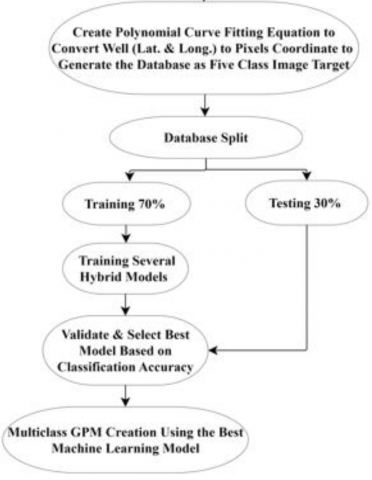
Figure 4. Well locations for machine learning model
The main difference between image and remote sensing data is that remote sensing (raster data) is linked to a geographical reference frame, location on the earth's surface indicated by Lat. and Long. In contrast, the spatial coordinates of pixels indicate image data. Therefore, the next step in data pre-processing is to create an equation to convert well latitude and longitude coordinates into the pixel coordinates for images using polynomial curve fitting to create the database for the collected wells that contain the features of thematic maps and the classes of the pumping rate. Polyfit function used to find the coefficients of a polynomial that fits a set of data which is mathematically expressed in Eq. (1) [21]:
$\mathrm{p}=$ Polyfit $(x, y, n)$ (1)
where, x and y are vectors containing the x and y coordinates of the data points, n is the degree of the polynomial to fit. After obtaining the polynomial for the fit line using the Polyfit function, the Polyval function can be used to evaluate the polynomial (p) at additional locations in (x), which is described as:
y= Polyval $(p, x)$ (2)
The generated equations using Polyfit and Polyval functions are:
$\mathrm{x}=-0.0017 \times \mathrm{y}_1+6.127 \mathrm{e}+03$ (3)
$y=0.0017 \times x_1-3.025 e+02$ (4)
There were five classes of image targets identified based on the available data for wells' discharge rates: (very poor) for pumping rates below 3 l/sec, (poor) for pumping rates between 4 and 6 l/sec, (moderate) for pumping rates between 7 and 9 l/sec, (good) for pumping rate between 10 and 14 l/sec and (very good) for pumping rates above 14 l/sec. Each thematic map feature in the database was multiplied by its weight, as presented in Table 1, to create a hybrid model that could effectively forecast groundwater potential zones and improve their management efficiency.
2.4 Classifier training
To properly train and assess available data, it is essential to divide the database into independent groups: Training data is used to determine the best parameters and classification models. On the other hand, testing data is used to objectively evaluate the predictive capabilities of trained classifiers [22]. The ratio for splitting the datasets is 70:30; 70% of the database is used for training the classifier model, while 30% is used as testing data to check the model's accuracy.
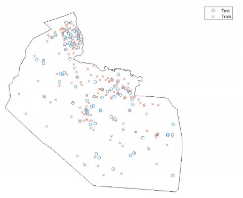
In geospatial data, it is common to find that closer observations have a stronger relationship than observations farther away [23]. MLAs are provided with the required information linking the location of the wells with the groundwater classes whenever spatial coordinates are used as input data for training and prediction. The combination of spatial values and a random distribution of samples over the whole study area will achieve an accurate machine-learning model when using testing data, according to Figure 5, which illustrates the distribution of water wells for the 70:30 splitting ratio. Hence, the total number of randomly selected wells was (242) and (107) for the training and validation process, respectively. It can be seen that the training data points sufficiently covered the study area.
Ultimately, the aim is to train a classification model that adequately fits the inputted training data and generalizes well to data that the MLA is unfamiliar with. One significant and non-trivial step in MLA classifier training is setting parameters appropriate for the particular task based on the available information [24].
2.5 Predictions evaluations
Testing data should be independent of the data used for training the classification machine learning model, ensuring a direct and statistically accurate indicator of the predicted performance of an achieved trained classifier [20]. While the output of classification models is discrete, we want a comparative measure for discrete classes. Classification metrics evaluate a model's performance and reveal the classification's accuracy in several ways. Metrics are used to monitor and assess the performance of a model during training and testing [25]. In this study, the Positive Rates (TPR), False Negative Rates (FNR), Positive Predictive Values (PPV), False Discovery Rates (FDR), the Area Under the Curve of the Receiver Operating Characteristics (ROC), and classifier accuracy were employed to evaluate the performance of classification learner. In the case of MLA-supervised classifiers, the generated categorical predictions may be evaluated using a confusion matrix, also known as an error matrix, as shown in Figure 6.
A confusion matrix provides a tabularized representation of the classification model's performance. The confusion matrix has the same number of rows and columns as the number of classes in the provided dataset.
The numbers in each matrix cell indicate the counts of class predictions for samples assigned to a specific category. The confusion matrix plot is used to understand how each class of the currently selected classifier is performed. It can be viewed after training the model from the plots section of the classification learner tab. The confusion matrix assists in identifying the areas in which the classifier has performed poorly. True Positive Rates (TPR) and False Negative Rates (FNR) were used to see how the classifier performed per true class. The TPR is the proportion of correctly classified observations per true class, while the FNR is the proportion of incorrectly classified observations per true class, as presented in Figure 7. Eqns. (5)-(6) provide a mathematical expression for the TPR and FNR, respectively [26]:
True Positive Rates $(\mathrm{TPR})=\frac{\mathrm{TP}}{\mathrm{TP}+\mathrm{FN}}$ (5)
False Negative Rates $(\mathrm{FNR})=\frac{\mathrm{FN}}{\mathrm{TP}+\mathrm{FN}}$ (6)
TP=true positives, FN=false negatives, and FP=false positives.
Figure 5. Training/testing data split model
Figure 6. Confusion matrix for five classes of machine learning model
Figure 7. The classifier performance per true class using True Positive Rates (TPR) and False Negative Rates (FNR)
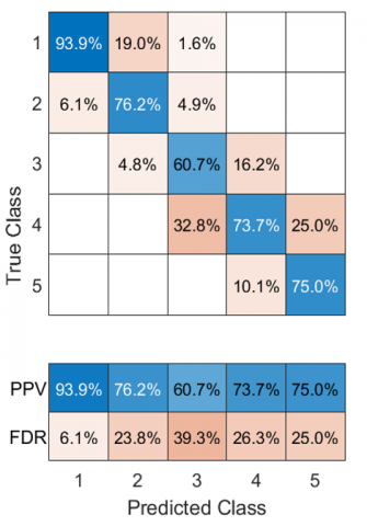
If false positives play an essential role in the classification issue, plot results were presented per predicted class instead of true class to investigate False Discovery Rates. Select the Positive Predictive Values (PPV) and False Discovery Rates (FDR) options to see results per predicted class. The positive predictive value, or PPV, indicates the percentage of observations properly identified for each predicted class. The false discovery rate, or FDR, is the fraction of poorly categorized observations for each predicted class. The Positive Predictive Values are shown in blue for the points in each class that was properly predicted, and the False Discovery Rates are displayed in orange for each class that was not correctly predicted. Figure 8 shows the classifier performance per predicted class using the Positive Predictive Values (PPV) and False Discovery Rates (FDR) options [21].
The Positive Predictive Values (PPV) and False Discovery Rates (FDR) are generally expressed as follows [26]:
Positive Predictive Values $(\mathrm{PPV})=\frac{\mathrm{TP}}{\mathrm{TP}+\mathrm{FP}}$ (7)
False Discovery Rates $(\mathrm{FDR})=\frac{\mathrm{FP}}{\mathrm{TP}+\mathrm{FP}}$ (8)
TP=true positives, FN=false negatives, and FP=false positives.
A Receiver Operating Characteristic (ROC) curve, which is a standard statistical tool, was used to evaluate the performance of the models by plotting sensitivity (TPR) and 1-specificity (FPR) on the y-axis and the x-axis, respectively calculated using Eqns. (9)-(10). The Area Under the Curve AUC measures the entire two-dimensional area underneath the ROC curve from (0,0) to (1,1), as shown in Figure 9. The values of AUC vary from 0 to 1. A model with 100% incorrect predictions has an AUC of 0.0, whereas one with 100% accurate predictions has an AUC of 1.0 [27].
sensitivity $=\frac{\mathrm{TP}}{\mathrm{TP}+\mathrm{FN}}$ (9)
1-specificity $=\frac{\mathrm{TN}}{\mathrm{TN}+\mathrm{FP}}$ (10)
TP=true positives, FN=false negatives, and FP=false positives.
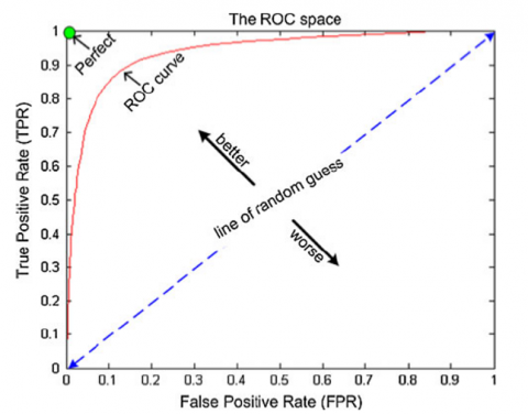
The value of FPR and TPR falls within the range [0, 1], and the green circle in the top left corner of Figure 10 indicates the best classification a classifier can achieve. Since then, (FPR, TPR) equal to (0.0,1.0) demonstrates that this classifier can correctly classify all data without making any false. The area under the ROC curve (AUC) is under the red curve [28].
The right angle to the upper left of the plot indicates a perfect outcome with no misclassified points. A poor result that is no better than random is a line at 45 degrees. The AUC number measures the overall quality of the classifier [26].
The final step in model development is the validation performance, calculated using model accuracy, using 30% of the dataset (testing data). Accuracy is a statistical metric that indicates how effectively a classifier can identify the different classes accurately and predict the unlabeled data. It is possible to compute the accuracy using the formula of Eq. (11), which refers to the percentage of true results (both true positive and true negative) in the dataset [29].
Accuracy $=\frac{\mathrm{TP}+\mathrm{TN}}{\mathrm{TP}+\mathrm{TN}+\mathrm{FP}+\mathrm{FN}}$ (11)
Figure 8. The classifier performance per predicted class using the Positive Predictive Values (PPV) and False Discovery Rates (FDR)
Figure 9. Area under the ROC curve [27]
Figure 10. ROC curve [28]
3.1 Assessment of models' predictive capability
A compression analysis is carried out for the predictive ability of the following five supervised machine learning algorithms: Ensemble Boosted Trees; Naive Bayes (NB); Support Vector Machines (SVM); Multi-Layer Perceptron (MLP), and k-Nearest Neighbours (kNN) was applied to the task of supervised classification using spatially constrained remotely sensed data. The performance of predictive models is evaluated using the metrics mentioned in section 2.5 of predictions evaluation.
3.1.1 Performance evaluation of Ensemble Boosted Trees-logic-based learners
Ensemble learning is a machine learning approach that involves training several learners to solve the same problem. Unlike traditional machine learning algorithms that attempt to learn a single hypothesis from training data, ensemble methods try to create and combine several theories. In data mining, classification algorithms can process significant information simultaneously. It is possible to establish assumptions about categorical class names, categorize information based on training sets and class labels, and classify newly obtained data using this method, mainly used for grouping purposes [30, 31]. In this case, the number of learners was equal to (30) with the learner type of decision tree. The maximum number of splits was (20) used to fit the model on the training set and evaluate it on the testing set. The accuracy of this model for training data is 72.3%. The confusion matrix plot is presented in Figure 11 to understand how the currently selected classifier is performed in each class and to identify the areas where the classifier has performed poorly.
The columns represent the predicted class, while the rows indicate the true (actual) class. The diagonal cells show where the true class and predicted class are matched. If the diagonal cells in this pattern are blue, the classifier correctly identifies the data in this true class, while classes with orange color are misclassified. On the other hand, the proportion of correctly classified observations per true class (TPR) and the proportion of incorrectly classified observations per true class (FNR) are presented in Figure 12. The last two columns on the right illustrate a percentage summary per true class. The correctly identified wells with pumping rates below 3 l/sec indicated as class 1 (very poor) are 47, as shown in Figure 11, while the misclassified classes are 4.
As a result, the TPR and FNR equal 92.2% and 7.8%, respectively, as presented in Figure 12 and calculated from Eqns. (5)-(6). In Figure 13, the result is plotted per predicted class instead of true class to investigate the False Discovery Rates FDR, the fraction of observations that were not properly categorized for each predicted class. Since the true positives (TP) observations are 47 well and false positives (FP) observations are 6 wells per predicted class. The Positive Predictive Values (PPV) and False Discovery Rates (FDR) are calculated as in Eqns. (7)-(8), which equals 88.7% and 11.3%, respectively.
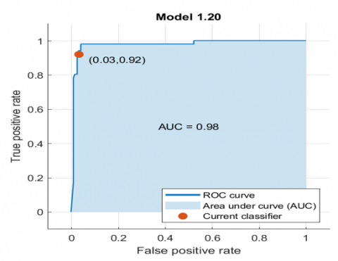
The Receiver Operating Characteristic (ROC) curve represents the model's performance after training. The ROC curve displays the provided trained classifier's true positive and false positive rates. The optimal solution is a right angle that reaches the upper left corner of the plot since there are no misclassified points. A poor result may be found below a line sloped at 45 degrees, referred to as the line of a random guess. The number that represents the Area Under the Curve is a measurement of the overall quality of the classifier. The larger area under curve values indicates better classifier performance. The AUC for the Ensemble Boosted Trees model is equal to (0.98), as presented in Figure 14.
Figure 11. Confusion matrix of Ensemble Boosted Trees model
Figure 12. Ensemble Boosted Trees model performance per true class using True Positive Rates (TPR) and False Negative Rates (FNR)
Figure 13. Ensemble Boosted Trees model performance per predicted class using the Positive Predictive Values (PPV) and False Discovery Rates (FDR)
Figure 14. ROC curve of the Ensemble Boosted Trees model
Figure 15. Confusion matrix of testing data for the Ensemble Boosted Trees model
Finally, the model is tested using the 30% of remaining data that is not involved in model building and training. The accuracy of the Ensemble Boosted Trees model is calculated using Eq. (11) from the confusion matrix of the testing data as the percentage of true results in the dataset's diagonal cells (true positive and true negative) to the total number of (107) testing wells, which is equal to 89.7%, as presented in Figure 15, where R stands for the confusion matrix of the testing data and (ans) denotes the calculated accuracy value.
3.1.2 Performance evaluation of support vector machine (SVM) algorithms
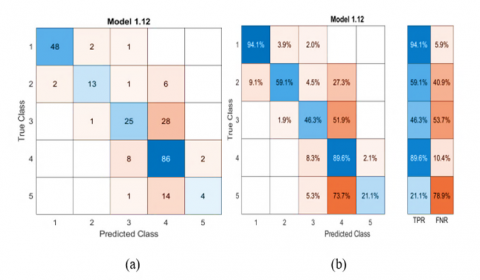
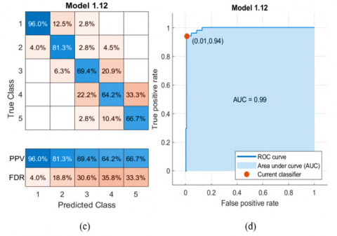
By using kernel functions, the Support Vector Machine (SVM) can locate nonlinear decision boundaries [32]. There are two primary steps. In the first step, the inputted original data are initially transformed into a space with a higher dimension using the kernel function (polynomial, Gaussian, radial basis function, exponential radial function, Multi-Layer Perceptron, etc.). The second step is searching for a hyperplane that linearly separates data in the new space [33]. In the current study, medium Gaussian SVM was applied for training data; the kernel function used for data transforming into the higher dimension to generate the Gaussian surface makes the data linearly separable. The accuracy of this model for training data is 72.7%. The performance of the SVM classification learning model was evaluated using the confusion matrix and the statistical metrics: True Positive Rates (TPR), False Negative Rates (FNR), Positive Predictive Values (PPV), False Discovery Rates (FDR), and AUC are presented in Figure 16. TPR and PPV should be high, and FNR and FDR should be low for better performance. The AUC of the SVM is (0.99). On the other hand, the SVM classifier's accuracy in the case of testing data was 77.6%.
Figure 16. Performance of the SVM classification learning model: (a) confusion matrix in the form of observations number; (b) TPR and FNR ratio; (c) PPV and FDR (d) ROC curve
3.1.3 Performance evaluation of Naive Bayes (NB)-statistical learning algorithms
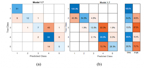
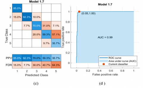
The methods in this category include Linear Discriminant Analysis (LDA) and Quadratic Discriminant Analysis (QDA), which employ density estimation strategies to identify linear (or quadratic) combinations of variables that optimally divide groups into separate categories [34]. The Gaussian Naive Bayes classifier was used for training data in this study. It is used for continuous numerical features. The distribution of continuous values is assumed to be Gaussian/normal distribution; it gives a bell-shaped curve that is symmetric about the mean of the feature values. And therefore, the probabilities are computed based on Gaussian distribution. The performance of the Naive Bayes (NB) classifier was evaluated, as presented in Figure 17.
The accuracy of this model for training data is 66.5%. Figure 17 (b) shows that the True Positive Rate (TPR) for class 1 is 100%, indicating a perfect outcome with no misclassified points; however, the TPR for classes 3 and 5 is lower than the (FNR); therefore, the data must be trained using another classifier that provides better performance.
The AUC of the Naive Bayes classifier is equal to 0.99. In comparison, the accuracy of the current classifier for testing data is 75.7%.
Figure 17. Performance of the Naive Bayes classification learning model: (a) confusion matrix of observations number; (b) TPR and FNR ratio; (c) PPV and FDR; (d) ROC curve
3.1.4 Performance evaluation of Multi-Layer Perceptron (MLP)-Artificial Neural Networks (ANN)
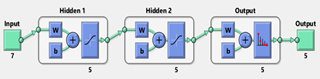
Perceptron is an algorithm for supervised learning consisting of four major components: input values, weights and biases, net sum, and an activation function; Figure 18 presents these principal components, a weighted sum of inputs followed by an activation function that can be generalized to the form of:
$\mathrm{y}_{\mathrm{i}}=\mathrm{f}_{\mathrm{k}}\left(\sum_{\mathrm{i}} \mathrm{W}_{\mathrm{i}} \mathrm{X}_{\mathrm{i}}\right)$ (12)
where, Wji represents the weight that may be adjusted for the ith instance and Xi represents one of the variables that are supplied. The activation function, denoted by fk, may take the form of any nonlinear function, such as a step function or a sigmoidal function [23].
The trained MLP neural network of five class classification was formed by an input layer with seven neurons representing the seven data features of the thematic maps for the affecting factors of the groundwater potential map, two hidden layers with five neurons in each layer, and an output layer with five neurons. The output layer performs the required task, such as prediction and classification. The target of the network was indicated by the neurons that are output. The neurons in the MLP were trained with the backpropagation learning algorithm, and the hyperbolic tangent function is the activation function of the hidden layers. The softmax transfer function was used inside the output layer. Because of its ability to convert input data into probability, this transfer function is often used in the output layer of classified Artificial Neural Networks (ANN). The softmax normalizes an input value into values that follow a probability distribution totaling up to 1. It is preferred in the multi-class classification of the neural network model because the output values are in the range [0,1], unlike the binary classification, which can only accept the value 0 or 1. In the case of small or negative inputs, the softmax turns it into a small probability, and if the input is large, it turns it into a large probability, but it will always remain between 0 and 1 [35].
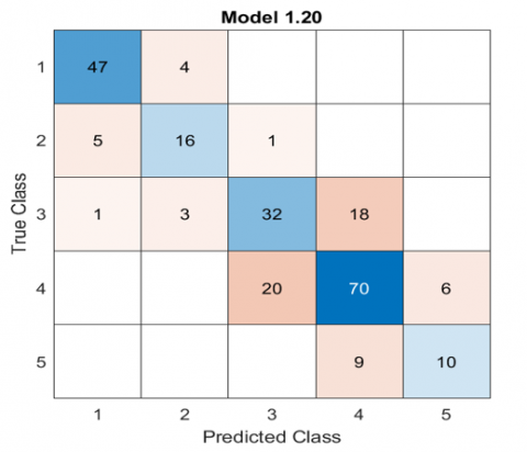
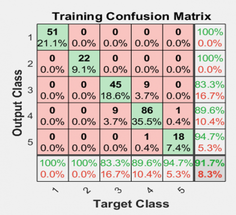
The accuracy of correct classified classes is 91.7% for (100000) epoch/iterations; the training confusion matrix of the MLP neural network is shown in Figure 19.
The rows represent the predicted neural network class (the output class), whereas the columns represent the actual class (target class). The observations that have been successfully categorized are shown by the diagonal cells. The observations that were not correctly categorized are shown by the off-diagonal cells. Each cell displays the overall number of observations and a percentage of the total observations. The percentage numbers shown in green reflect the proportion of correctly classified observations to the total observations.
In contrast, the percentages displayed in red represent the proportion of data incorrectly classified. The column on the far right of Figure 19 displays the percentages of all the predicted samples to belong to each class that was correctly and incorrectly classified. These metrics are often called the precision (or positive predictive value) for correctly classified classes and the false discovery rate for the incorrectly classified classes. The row at the bottom of the graph shows the proportion of samples properly and wrongly identified for each target class. Recall (or true positive rate) and false negative rate are common names for these statistics. The total accuracy is shown in the cell located in the plot's bottom right corner (91.7%).
Acceptable results are achieved due to the almost complete straightening ROC curve for classes 3 and 4, as presented in Figure 20.
When the area under the ROC curve is closer to the value 1 or when the ROC curve straightened at the top of the graph in the case of 100% of TPR (sensitivity) and 100% of FPR (specificity), performance levels are considered to be at their highest. Hence, the performance of classifications developed by ANN provides a perfect result for classes 1, 2 and 5. Finally, the model is tested using a 30% testing dataset to calculate the model accuracy, which was 79.4%.
Figure 18. Structure of proposed five-class MLP neural network
Figure 19. Training confusion matrix of the MLP neural network
Figure 20. Training ROC curve for MLP neural network model
3.1.5 Performance evaluation of k-Nearest Neighbours (kNN)-instance-based learners
The k-Nearest Neighbors (kNN) method is a non-parametric supervised learning technique. In this study, we investigate the impact of distance metrics while using kNN as the classifier for image classification. Non-parametric algorithms mean it makes no assumptions about the data distribution [36]. When working with KNN, the distance between two data points is determined by a similarity measure, also known as a distance function. The Euclidean distance was used in this model, generated from a generalized metric known as Minkowski distance. As p=2, Minkowski distance is specific to Euclidean distance. The majority vote of the closest sample classes identifies the sample's class [34].
The weighted kNN with the number of neighbors equal to (10) was used to train the dataset. The accuracy of the trained model is 93.0%. Figure 20 shows the current model's performance. The total number of misclassified cells is (17) knowing the total number of the trained dataset is (242).
The wells of classes 1 and 2 are perfectly classified (100%) of TPR and (0%) of FNR, while for classes 3, 4 and 5, the TPR was equal to (88.9%, 90.6%, and 89.5%) respectively. On the other hand, the kNN classifier's accuracy in the testing phase was equal to 90.7%.
The best classifier for accurate groundwater potential zone mapping was determined by comparing the predictive abilities of five machine-learning techniques using the classifier's performance accuracy and some metrics, including True Positive Rates (TPR), False Negative Rates (FNR), Positive Predictive Values (PPV), False Discovery Rates (FDR), and the Area Under the Curve of the Receiver Operating Characteristics (ROC). The k-Nearest Neighbours (kNN)-instance-based learners are the best machine learning models in the training and testing phase due to their classification accuracy (93.0% and 90.7%), respectively. In addition, the TPR is much higher than FNR, which indicates better performance for the kNN classifier. From the ROC curve presented in Figure 21 (d), it can be noticed that the area under curve AUC that measures the entire two-dimensional area underneath the ROC curve is 1 with (false positive rate, true positive rate) equal to (0,1), which indicates 100% accurate predictions. Thus, the groundwater potential map shown in Figure 22 was created using this model. Also, Figure 23 shows the percentage of groundwater areal distribution for the very poor, poor, moderate, good, and very good groundwater zones: (5.58%, 4.24%, 35.69%, 42.12%, and 12.37%), respectively.
Figure 21. Performance of k-Nearest Neighbors (kNN) model: (a) confusion matrix of observations number; (b) TPR and FNR ratio; (c) PPV and FDR (d) ROC curve
Figure 22. GPM using the k-Nearest Neighbours (kNN) classifier
Figure 23. Percentage of areal distribution for groundwater potential zones (GWPZ)
The groundwater potential zones (GWPZs) in the southern desert of Iraq along the Najaf and Muthanna governorates are identified in this study, applying remote sensing (RS), geographic information system (GIS), and analytical hierarchy process (AHP) methods. With the help of published maps for soil and main groundwater aquifers units, Rs data (satellite images and STRM DEM), data from groundwater wells, and assigned weights and ranks for groundwater potentiality influencing factors and their respective classes using the AHP technique, thematic layers of aquifer unit types, transmissivity, lineaments density, slope, soil type, land use and cover, and drainage density were prepared. The prepared thematic layers were used as input variables for MLAs, and the collected data from (349) groundwater wells were used to train and evaluate the five developed hybrid ML models. The True Positive Rates (TPR), False Negative Rates (FNR), Positive Predictive Values (PPV), False Discovery Rates (FDR), the Area Under the Curve (AUC) of the Receiver Operating Characteristics (ROC), and the accuracy of the classifier are used to assess the performance of ML models. According to the analysis of ML models and based on their accuracy matrices, the results show that all developed models are highly predictive, but the k-Nearest Neighbors (kNN) model is the most effective at identifying areas with significant groundwater potential with an accuracy of 90.70%, followed by Ensemble Boosted Trees-Logic-Based Learners, Multi-Layer Perceptron (MLP)-Artificial Neural Networks (ANN), Support Vector Machine (SVM), and Naive Bayes (NB)-Statistical Learning Algorithms with validation accuracy of (89.7%, 79.4%, 77.6%, and 75.7%) respectively. In addition, the total number of misclassified cells is (17) in the kNN model, given that the training dataset size is (242). Class 1 and 2 wells are ideally rated (100% TPR and 0% FNR), while classes 3-5 had TPRs of 89%, 90%, and 89.5%.
Consequently, a five-class groundwater potential map is created using the k-Nearest Neighbors (kNN): (very poor) for pumping rates below 3 l/sec, (poor) for pumping rates between 4 and 6 l/sec, (moderate) for pumping rates between 7 and 9 l/sec, (good) for pumping rate between 10 and 14 l/sec and (very good) for pumping rates above 14 l/sec. According to the findings, there are five different groundwater potential zones (GWPZ): very poor (4281.69Km2), poor (3253.47Km2), moderate (27385.90Km2), good GWPZ (32319.82Km2), and very good (9491.84Km2).
The developed hybrid model can accurately predict the state of groundwater potential zones and allows the opportunity to characterize the behavior of a groundwater source by integrating the effect of the set of influencing factors represented by the seven thematic maps with their respective effect weights. Also, it can be modified with new data. Also, the process used in the present research could be applied and evaluated in other areas to produce GPMs. In brief, GPMs might greatly assist water resource managers and planners in understanding water resources' conditions, exploitation, and conservation measures.
This work is supported by the General Commission of Groundwater, Ministry of Water Resources, Iraq, which provided the data needed to complete this research.
|
DEM |
Digital elevation model |
|
SRTM |
Shuttle radar topography mission |
|
RS |
Remote sensing |
|
GIS |
Geographic information system |
|
AHP |
Analytical hierarchy process |
|
GPM |
Groundwater potential map |
|
GWPZ |
Groundwater potential zone |
|
MLAs |
Machine learning algorithms |
|
NB |
Naive Bayes |
|
SVM |
Support Vector Machines |
|
MLP |
Multi-Layer Perceptron |
|
ANN |
Artificial Neural Networks |
|
kNN |
k-Nearest Neighbours |
|
GPM |
Groundwater potential map |
|
GWPZ |
Groundwater potential zone |
|
TPR |
True Positive Rates |
|
FNR |
False Negative Rates |
|
PPV |
Positive Predictive Values |
|
FDR |
False Discovery Rates |
|
AUC |
Area under curve |
|
ROC |
Receiver Operating Characteristics |
|
LDA |
Linear discriminant analysis |
|
QDA |
Quadratic discriminant analysis |
[1] Díaz-Alcaide, S., Martínez-Santos, P., Villarroya, F. (2017). A commune-level groundwater potential map for the Republic of Mali. Water, 9(11): 839. https://doi.org/10.3390/w9110839
[2] Jha, M.K., Chowdary, V.M., Chowdhury, A. (2010). Groundwater assessment in Salboni Block, West Bengal (India) using remote sensing, geographical information system and multi-criteria decision analysis techniques. Hydrogeology Journal, 18(7): 1713-1728. https://doi.org/10.1007/s10040-010-0631-z
[3] Díaz-Alcaide, S., Martínez-Santos, P. (2019). Review: Advances in Groundwater Potential Mapping. Hydrogeology Journal, 27(7): 2307-2324. https://doi.org/10.1007/s10040-019-02001-3
[4] Rahmati, O., Nazari Samani, A., Mahdavi, M., Pourghasemi, H.R., Zeinivand, H. (2015). Groundwater Potential Mapping at Kurdistan region of Iran using analytic hierarchy process and GIS. Arabian Journal of Geosciences, 8: 7059-7071. https://doi.org/10.1007/s12517-014-1668-4
[5] Yin, H.Y., Shi, Y.L., Niu, H.G., Xie, D.L., Wei, J.C., Lefticariu, L., Xu, S.X. (2017). A GIS-based model of potential groundwater yield zonation for a sandstone aquifer in the Juye Coalfield, Shangdong, China. Journal of Hydrology, 557: 434-447. https://doi.org/10.1016/j.jhydrol.2017.12.043
[6] Al-Djazouli, M.O., Elmorabiti, K., Rahimi, A., Amellah, O., Fadil, O.A.M. (2021). Delineating of groundwater potential zones based on remote sensing, GIS and analytical hierarchical process: A case of Waddai, eastern Chad. GeoJournal, 86: 1881-1894. https://doi.org/10.1007/s10708-020-10160-0
[7] Gómez-Escalonilla, V., Martínez-Santos, P., Martín-Loeches, M. (2022). Preprocessing approaches in machine-learning-based Groundwater Potential Mapping: An application to the Koulikoro and Bamako regions, Mali. Hydrology and Earth System Sciences, 26(2): 221-243. https://doi.org/10.5194/hess-26-221-2022
[8] Mohr, F., Wever, M., Hüllermeier, E. (2018). ML-Plan: Automated machine learning via hierarchical planning. Machine Learning, 107: 1495-1515. https://doi.org/10.1007/s10994-018-5735-z
[9] Da Silva, I.N., Hernane Spatti, D., Andrade Flauzino, R., Liboni, L.H.B., dos Reis Alves, S.F. (2017). Artificial neural network architectures and training processes. Artificial Neural Networks, A Practical Course, Springer International Publishing, 21-28. https://doi.org/10.1007/978-3-319-43162-8_2
[10] Agatonovic-Kustrin, S., Beresford, R. (2000). Basic concepts of artificial neural network (ANN) modeling and its application in pharmaceutical research. Journal of pharmaceutical and Biomedical Analysis, 22(5): 717-727. https://doi.org/10.1016/S0731-7085(99)00272-1
[11] Ozdemir, A. (2011). Using a binary logistic regression method and GIS for evaluating and mapping the groundwater spring potential in the Sultan Mountains (Aksehir, Turkey). Journal of Hydrology, 405(1-2): 123-136. https://doi.org/10.1016/j.jhydrol.2011.05.015
[12] Nguyen, P.T., Ha, D.H., Jaafari, A., Nguyen, H.D., Van Phong, T., Al-Ansari, N., Prakash, I, Van Le, H., Pham, B.T. (2020). Groundwater Potential Mapping combining artificial neural network and real AdaBoost ensemble technique: The DakNong province case-study, Vietnam. International Journal of Environmental Research and Public Health, 17(7): 2473. https://doi.org/10.3390/ijerph17072473
[13] Sarkar, S.K., Talukdar, S., Rahman, A., Shahfahad, Roy, S.K. (2022). Groundwater potentiality mapping using ensemble machine learning algorithms for sustainable groundwater management. Frontiers in Engineering and Built Environment, 2(1): 43-54. https://doi.org/10.1108/FEBE-09-2021-0044
[14] Phong, T.V., Pham, B.T., Trinh, P.T., Ly, H.B., Vu, Q.H., Ho, L.S., Van Le, H., Phong, L.H., Avand, M., Prakash, I. (2021). Groundwater Potential Mapping using GIS-based hybrid artificial intelligence methods. Groundwater, 59(5): 745-760. https://doi.org/10.1111/gwat.13094
[15] Tamiru, H., Wagari, M., Tadese, B. (2022). An integrated artificial intelligence and GIS spatial analyst tools for delineation of groundwater potential zones in complex terrain: Fincha catchment, Abay Basi, Ethiopia. Air, Soil and Water Research, 15: 1-15. https://doi.org/10.1177/11786221211045972
[16] Sissakian, V.K., Youkhana, R.Y., Zainal, E.M. (1994). The geology of Al-Birreet Quadrangle NH-38-1, Scale 1: 250 000. Geosurv. Baghdad, Iraq.
[17] Messene, G.M. (2017). Groundwater flow direction, recharge and discharge zones identification in lower Gidabo Catchment, Rift Valley Basin, Ethiopia. Journal of Environment and Earth Science, 7: 32-39. https://www.iiste.org/Journals/index.php/JEES/article/view/35430.
[18] Al-Jiburi, H.K., Al-Basrawi, N.H. (2007). Hydrogeology. Iraqi Bulletin of Geology and Mining, Special Issue: Geology of Iraqi Western Desert, (1): 125-144.
[19] Luijendijk, E. (2022). Transmissivity and groundwater flow exert a strong influence on drainage density. Earth Surface Dynamics, 10(1): 1-22. https://doi.org/10.5194/esurf-10-1-2022
[20] Guyon, I. (2009). A practical guide to model selection. Proc. Mach. Learn. Summer School Springer Text Stat, 1-37.
[21] MATLAB. (2020). Version 9.9.0.1467703 (R2020b). Natick, Massachusetts: The MathWorks Inc.
[22] Hastie, T., Tibshirani, R. Friedman, J. (2009). The elements of statistical learning: Data mining, inference and prediction, second edition. Springer Series in Statistics, New York: Springer, 2: 1-758.
[23] Getis, A. (2009). Spatial autocorrelation. In Handbook of Applied Spatial Analysis: Software Tools, Methods and Applications. Berlin, Heidelberg: Springer Berlin Heidelberg, 255-278. https://doi.org/10.1007/978-3-642-03647-7_14
[24] MacKay, D.J.C. (2003). Information Theory, Inference, and Learning Algorithms. Cambridge University Press, Cambridge, 640.
[25] Vujović, Ž. (2021). Classification model evaluation metrics. International Journal of Advanced Computer Science and Applications (IJACSA), 12(6): 599-606. https://doi.org/10.14569/IJACSA.2021.0120670
[26] Vihinen, M. (2012). How to evaluate performance of prediction methods? Measures and their interpretation in variation effect analysis. In BMC Genomics, 13(4): 1-10. https://doi.org/10.1186/1471-2164-13-S4-S2
[27] Kuruvilla, J., Gunavathi, K. (2014). Lung cancer classification using neural networks for CT images. Computer Methods and Programs in Biomedicine, 113(1): 202-209. https://doi.org/10.1016/j.cmpb.2013.10.011
[28] Amin, M.A., Yan, H. (2011). High speed detection of retinal blood vessels in fundus image using phase congruency. Soft Computing, 15: 1217-1230. https://doi.org/10.1007/s00500-010-0574-2
[29] Ling, Y., Mahadevan, S. (2013). Quantitative model validation techniques: New insights. Reliability Engineering & System Safety, 111: 217-231. https://doi.org/10.1016/j.ress.2012.11.011
[30] Nikam, S.S. (2015). A comparative study of classification techniques in data mining algorithms. Oriental Journal of Computer Science and Technology, 8(1): 13-19.
[31] Gavankar, S.S., Sawarkar, S.D. (2017). Eager decision tree. In 2017 2nd International Conference for Convergence in Technology (I2CT), IEEE, 837-840. https://doi.org/10.1109/I2CT.2017.8226246
[32] Hsu, C.W., Lin, C.J. (2002). A comparison of methods for multiclass Support Vector Machines. In IEEE Transactions on Neural Networks, 13(2): 415-425. https://doi.org/10.1109/72.991427
[33] Melgani, F., Bruzzone, L. (2004). Classification of hyperspectral remote sensing images with Support Vector Machines. In IEEE Transactions on Geoscience and Remote Sensing, 42(8): 1778-1790. https://doi.org/10.1109/TGRS.2004.831865
[34] Kotsiantis, S.B. (2007). Supervised machine learning: A review of classification techniques. Emerging Artificial Intelligence Applications in Computer Engineering, 160(1): 3-24.
[35] Nwankpa, C., Ijomah, W., Gachagan, A., Marshall, S. (2018). Activation functions: Comparison of trends in practice and research for deep learning. arXiv preprint arXiv:1811.03378. https://doi.org/10.48550/arXiv.1811.03378
[36] Zhang, M.L., Zhou, Z.H. (2007). ML-KNN: A lazy learning approach to multi-label learning. Pattern Recognition, 40(7): 2038-2048. https://doi.org/10.1016/j.patcog.2006.12.019