Sirasrete Phoosree![]() | Onuma Suphattanakul
| Onuma Suphattanakul![]() | Ekarach Maliwan
| Ekarach Maliwan![]() | Marisa Senmoh
| Marisa Senmoh![]() | Weerachai Thadee*
| Weerachai Thadee*![]()
© 2023 IIETA. This article is published by IIETA and is licensed under the CC BY 4.0 license (http://creativecommons.org/licenses/by/4.0/).
OPEN ACCESS
The nonlinear space and time fractional (2+1)-dimensional cubic Klein-Gordon (cKG) equation and the nonlinear space and time fractional (2+1)-dimensional Gardner-KP (GKP) equation are applied to model crystal dislocation and internal waves on ocean shelves, respectively. To solve these equations, the fractional cKG and GKP equations are first converted into nonlinear ordinary differential equations (ODEs) using wave transformation and Jumarie's Riemann-Liouville derivative. The solution is then expressed as a finite series, and this approach is combined with the generalized Bernoulli equation method. Exact traveling wave solutions are obtained in the form of exponential functions, hyperbolic functions, and rational functions, which ultimately give rise to physical waves. These waves manifest in various forms, such as kink, periodic, and solitary waves, and are represented by two-dimensional and three-dimensional graphical illustrations.
fractional partial differential equations, generalized Bernoulli equation method, traveling wave solution, fractional cubic Klein Gordon equation, fractional Gardner-KP equation
Nonlinear phenomena encompass a diverse range of applications, spanning fields such as atmospheric science, condensed matter physics, theoretical particle physics, and cosmic structures. These phenomena are particularly relevant in disciplines including fluid mechanical engineering, electrical engineering, solid-state physics, plasma physics, plasma waves, chemical physics, and optical fibers. Nonlinear waves and the structures they elucidate are central to contemporary theories across various domains. Nonlinear partial differential equations (PDEs) play a critical role in characterizing nonlinear wave phenomena, accounting for dispersion, dissipation, convection, and response. Current research efforts are primarily focused on exploring exact or numerical solutions to leverage the insights derived from these studies. Investigating the precise traveling wave solutions of nonlinear fractional PDEs is crucial for deepening our understanding of the underlying factors.
A myriad of methods has been employed to solve nonlinear fractional PDEs, including the Riccati-Bernoulli sub-ODE method [1, 2], Kudyashov [3, 4], first integral method [5, 6], generalized Kudryashov method [7, 8], modified Kudryashov method [9, 10], functional variable method [11, 12], G′/G-expansion method [13, 14], fractional sub-equation method [15, 16], and simple equation method [17, 18].
In 2006, the Riemann-Liouville derivative of the Jumarie equation [19] was described as follows:
$D_{t}^{\alpha }\Upsilon \left( t \right)=\left\{ \begin{array}{*{35}{l}} \Upsilon \left( t \right) & ,\alpha =0 \\ \frac{\frac{d}{dt}\int\limits_{0}^{t}{\frac{\left[ \Upsilon \left( \delta \right)-\Upsilon \left( 0 \right) \right]}{{{\left( t-\delta \right)}\quad ^{\alpha }}}\quad d\delta }}{\Gamma \left( 1-\alpha \right)} & ,0<\alpha <1 \\ \frac{{{d}^{n}}}{d{{t}^{n}}}D_{t}^{\alpha -n}\Upsilon \left( t \right) & \begin{align} & ,n\le \alpha <n+1, \\ & n\ge 1, \\\end{align} \\\end{array} \right.$ (1)
where, a is an order of the fractional derivative.
In 2009, the following was presented as the Riemann-Liouville derivative of the Jumarie [20]:
$D_{t}^{\alpha }{{t}^{\varphi }}=\frac{\Gamma \left( \varphi +1 \right)}{\Gamma \left( \varphi -\alpha +1 \right)}{{t}^{\varphi -\alpha }},\,\,\varphi \ge 0,$ (2)
$D_{t}^{\alpha }\left[ \Upsilon \left( t \right)\Psi \left( t \right) \right]=\Upsilon \left( t \right)D_{t}^{\alpha }\Psi \left( t \right)+\Psi \left( t \right)D_{t}^{\alpha }\Upsilon \left( t \right),$ (3)
$D_{t}^{\alpha }\Upsilon \left[ \Psi \left( t \right) \right]=D_{\Psi }^{\alpha }\Upsilon \left[ \Psi \left( t \right) \right]{{\left[ {\Psi }'\left( t \right) \right]}^{\alpha }}={{{\Upsilon }'}_{\Psi }}\left[ \Psi \left( t \right) \right]D_{t}^{\alpha }\Psi \left( t \right).$ (4)
The (2+1)-dimensional cKG equation is one of the second-order non-linear evolution equations. This equation has been employed to form a variety of different non-linear phenomena [21], including the propagation of crystal dislocation, the action of elementary particles, and the proliferation of fluxions in Josephson junctions, to name a few examples. The cKG equation has a non-linearity that indicates that the constant value with ω=ω(x, y, t) and β, ε are not zero, as seen below:
${{\omega }_{xx}}+{{\omega }_{yy}}-{{\omega }_{tt}}+\beta \omega +\varepsilon {{\omega }^{3}}=0.$ (5)
The exact solution [21] of Eq. (5) is:
$\omega =\pm I\sqrt{\frac{\beta }{\varepsilon }}\left( 1-\frac{2{{b}_{1}}\cosh ({{b}_{2}})+sinh({{b}_{2}})}{({{b}_{1}}-2{{a}_{2}}\alpha )\cosh ({{b}_{2}})+({{b}_{1}}+2{{a}_{2}}\alpha )sinh({{b}_{2}})} \quad\right),$ (6)
where, $b_1=a_1\left(\lambda^2-2\right), b_2=\sqrt{\frac{\alpha}{-2\left(\lambda^2-2\right)}}(x+y-\lambda t)$ and a1, a2 are constants of integration.
On the ocean shelf, powerful nonlinear internal waves are described by the (2+1) dimensional GKP Equation [22]. This is the form of the non-linear positive GKP Equation [23] of the fourth-order with ω=ω(x, y, t):
${{\left( {{\omega }_{t}}+6\omega {{\omega }_{x}}+6\omega {}^{2}{{\omega }_{x}}+{{\omega }_{xxx}} \right)}_{x}}+{{\omega }_{yy}}=0.$ (7)
The explicit form of exact travelling wave solutions of positive GKP Equation [23] is:
$\omega=\frac{4(c+1) e^{\sqrt{-c-1 \,\,\xi}}}{4 c e^{2 \sqrt{-c-1} \,\,\,\,\xi}\,\,\,\,-4 e^{\sqrt{-c-1} \,\,\,\,\xi}\,\,\,\,\,-1}$, (8)
where, $\xi =\int{\frac{d\omega }{\varphi }},\,\,\varphi =\frac{d\omega }{d\xi }$ and c is wave speed.
The fractional cKG equation and the fractional GKP equation have both been solved in this article by using Jumarie's Riemann-Liouville derivative and the generalized Bernoulli equation method. We were able to get 13 solutions for each equation, and these solutions came in the form of hyperbolic functions, exponential functions, and rational functions. Using two-dimensional graphs and three-dimensional graphs, we were able to demonstrate the exact solutions as well as the physical waves which are kink waves, solitary waves and periodic waves. These results can be compared with the numerical solutions. Moreover, it can also be applied to initial and boundary value problems. Finding the traveling wave solutions in this research demonstrates the efficiency of the generalized Bernoulli equation method for solving the non-linear fractional PDEs.
We will go through the generalized Bernoulli equation method for solving fractional PDEs in this section. The fundamental form of fractional PDEs [24] may be illustrated as:
$F\left( \omega ,D_{x}^{\alpha }\omega ,D_{y}^{\alpha }\omega ,D_{t}^{\alpha }\omega ,D_{x}^{2\alpha }\omega ,D_{y}^{\alpha }D_{x}^{\alpha }\omega ,D_{t}^{\alpha }D_{x}^{\alpha }\omega ,\ldots \right)=0,$ (9)
where, t>0 and 0<α≤1.
The steps needed to carry out this procedure are outlined in the following instructions [24]:
Step 1: Wave transformation
The traveling wave solution to fractional partial differential equations is a solution that meets certain conditions.
$\omega \left( x,y,t \right)=\Theta \left( \delta \right),\,\delta =\frac{r{{x}^{\alpha }}}{\Gamma \left( \alpha +1 \right)}+\frac{s{{y}^{\alpha }}}{\Gamma \left( \alpha +1 \right)}-\frac{c{{t}^{\alpha }}}{\Gamma \left( \alpha +1 \right)},$ (10)
where, r and s are considered to be constants, c is also considered to be a constant, but this time it relates to the speed of the wave. Eq. (9) is converted into an ODE by Eq. (10):
$H\left( \Theta ,{\Theta }',{\Theta }'',{\Theta }''',\ldots \right)=0,$ (11)
where, H is a polynomial in $\Theta(\delta)$ and its derivatives.
Step 2: Solution supposition
We use the finite series to work out the solution to Eq. (11), and then we write it down:
$\Theta \left( \delta \right)=\sum\limits_{i=0}^{K}{{{b}_{i}}{{G}^{i}}\left( \delta \right)},$ (12)
where, bi are non-zero constants and G(δ) are variables that are dependent on using the method of the generalized Bernoulli equation, which states as follows:
${G}'\left( \delta \right)=\eta G\left( \delta \right)+\xi {{G}^{2}}\left( \delta \right),$ (13)
where, η, ξ are the constants that are not zero in the expression. The answers to Eq. (13) may be subdivided into 13 different situations [25].
For real and non-zero η, η2>0 and ξ≠0 the solutions to Eq. (13) are:
${{G}_{1}}\left( \delta \right)=\frac{-\eta -\eta \tanh \left( \frac{\eta \delta }{2} \right)}{2\xi },$ (14)
${{G}_{2}}\left( \delta \right)=\frac{-\eta -\eta \coth \left( \frac{\eta \delta }{2} \right)}{2\xi },$ (15)
${{G}_{3}}\left( \delta \right)=\frac{-\eta -\eta \tanh \left( \eta \delta \right)\mp i\eta \operatorname{sech}\left( \eta \delta \right)}{2\xi },$ (16)
${{G}_{4}}\left( \delta \right)=\frac{-\eta -\eta \coth \left( \eta \delta \right)\mp \eta \operatorname{csch}\left( \eta \delta \right)}{2\xi },$ (17)
${{G}_{5}}\left( \delta \right)=\frac{-2\eta -\eta \tanh \left( \frac{\eta \delta }{4} \right)-\eta \coth \left( \frac{\eta \delta }{4} \right)}{4\xi },$ (18)
${{G}_{6}}\left( \delta \right)=\frac{\eta \sqrt{{{Q}^{2}}+{{R}^{2}}}-\eta Q\cosh \left( \eta \delta \right)}{2\xi Q\sinh \left( \eta \delta \right)+2\xi R}-\frac{\eta }{2\xi },$ (19)
${{G}_{7}}\left( \delta \right)=\frac{-\eta \sqrt{{{R}^{2}}-{{Q}^{2}}}-\eta Q\sinh \left( \eta \delta \right)}{2\xi Q\cosh \left( \eta \delta \right)+2\xi R}-\frac{\eta }{2\xi },$ (20)
where, Q and R are two non-zero real constant that satisfy R2-Q2>0.
${{G}_{8}}\left( \delta \right)=\frac{\pm \eta {{e}^{\eta \delta }}}{\xi \mp \xi {{e}^{\eta \delta }}}\quad,$ (21)
${{G}_{9}}\left( \delta \right)=\frac{\pm \eta {{e}^{\eta \delta }}}{\xi i\mp \xi {{e}^{\eta \delta }}}\quad,$ (22)
${{G}_{10}}\left( \delta \right)=\frac{\eta \sqrt{{{Q}^{2}}-{{R}^{2}}}\pm \eta \left( Q{{e}^{\eta \delta }}-iR \right)}{\mp \xi Q\left( {{e}^{\eta \delta }}-{{e}^{-\eta \delta\quad }} \right)\pm 2\xi iR},$ (23)
where, Q and R are two non-zero real constant that satisfy ${{Q}^{2}}-{{R}^{2}}>0.$
${{G}_{11}}\left( \delta \right)=\frac{-\eta \phi {{e}^{\eta \delta }}}{\xi +\xi \phi {{e}^{\eta \delta }}}$ , (24)
${{G}_{12}}\left( \delta \right)=\frac{-\eta {{e}^{\eta \delta }}}{\xi \phi +\xi {{e}^{\eta \delta }}}$ , (25)
where, ϕ is an arbitrary constant.
For η=0 and ξ≠0 and arbitrary constant ψ, the solution to Eq. (13) is:
${{G}_{13}}\left( \delta \right)=\frac{-1}{\xi \delta +\psi }.$ (26)
Step 3: Finding the integer K
In order to get the integer K in Eq. (12), you must first strike a balance between the terms for the highest order derivative and the non-linear terms.
Step 4: Solution obtaining
Discover the values of the parameters bi, i=1, 2, 3, …, n and c by summing the coefficients of all expressions that have the same order as Gi(δ) and then setting those coefficients to zero. As a consequence of this, we make up the analytical solutions to Eq. (9).
Solving the two non-linear space-time fractional equations that are presented below allows us to show the generalized Bernoulli equation method.
Solving the two non-linear space-time fractional equations that are presented below allows us to show the generalized Bernoulli equation method.
3.1 The non-linear space and time fractional of (2+1)-dimensional cKG equation
The results of applying the non-linear space and time fractional cKG equation to traveling waves are shown below:
$D_{x}^{2\alpha }\omega +D_{y}^{2\alpha }\omega -D_{t}^{2\alpha }\omega +\beta \omega +\varepsilon {{\omega }^{3}}=0,$ (27)
when, t>0, 0<α≤1, ω=ω(x, y, t) and the value of β, ε are constants. Taking the assumption that ω(x, y, t)=$\Theta$(δ) is the correct result and applying transformation:
$\delta =\frac{r{{x}^{\alpha }}}{\Gamma \left( \alpha +1 \right)}+\frac{s{{y}^{\alpha }}}{\Gamma \left( \alpha +1 \right)}-\frac{c{{t}^{\alpha }}}{\Gamma \left( \alpha +1 \right)},$ (28)
where, the constants r, s and c do not have the value zero. Eq. (28) was used to develop an ODE:
${{r}^{2}}{\Theta }''+{{s}^{2}}{\Theta }''-{{c}^{2}}{\Theta }''+\beta \Theta +\varepsilon {{\Theta }^{3}}=0.$ (29)
Eq. (10) was the structure that was used in order to provide the solution to the issue by using the generalized Bernoulli equation method. After that, we made certain that the highest order derivative and the non-linear components of Eq. (29) were in balance with one another. Thus K=1. In the end, Eq. (12) was transformed into:
$\Theta \left( \delta \right)={{b}_{0}}+{{b}_{1}}G\left( \delta \right).$ (30)
Eq. (30) will take the place of Eq. (29) in this application. In order to make each coefficient equal to zero, we collected all of the terms that belonged to the same power of G(δ), and then we did the following:
${{G}^{0}}\left( \delta \right)\,\,\,\,\,:\,\,\,\,\,{{b}_{0}}\beta +b_{0}^{3}\varepsilon =0,$ (31)
${{G}^{1}}\left( \delta \right)\,\,\,\,\,:\,\,\,\,\,{{b}_{1}}{{r}^{2}}{{\eta }^{2}}+{{b}_{1}}{{s}^{2}}{{\eta }^{2}}-{{b}_{1}}{{c}^{2}}{{\eta }^{2}}+{{b}_{1}}\beta +3b_{0}^{2}{{b}_{1}}\varepsilon =0,$ (32)
${{G}^{2}}\left( \delta \right)\,\,\,\,\,:\,\,\,\,\,3{{b}_{1}}{{r}^{2}}\eta \xi +3{{b}_{1}}{{s}^{2}}\eta \xi -3{{b}_{1}}{{c}^{2}}\eta \xi +3{{b}_{0}}b_{1}^{2}\varepsilon =0,$ (33)
${{G}^{3}}\left( \delta \right)\,\,\,\,\,:\,\,\,\,\,2{{b}_{1}}{{r}^{2}}{{\xi }^{2}}+2{{b}_{1}}{{s}^{2}}{{\xi }^{2}}-2{{b}_{1}}{{c}^{2}}{{\xi }^{2}}+b_{1}^{3}\varepsilon =0.$ (34)
After working out the solution to the system of Eqns. (31)-(34), we obtain:
${{b}_{0}}=\pm \sqrt{-\frac{\beta }{\varepsilon }},$ (35)
${{b}_{1}}=\pm \xi \sqrt{-\frac{2\left( {{r}^{2}}+{{s}^{2}}-{{c}^{2}} \right)}{\varepsilon }},$ (36)
$c=\pm \frac{\sqrt{{{r}^{2}}{{\eta }^{2}}+{{s}^{2}}{{\eta }^{2}}-2\beta }}{\eta }.$ (37)
Eqns. (14)-(26), (28), and (35)-(37) provide for the representation of the exact traveling wave solutions of the non-linear space-time fractional cKG equations in a total of 13 different cases which are distinct from the one that was found in the first solution indicated in Eq. (6).
For real and non-zero η, η2>0 and ξ≠0a and let ${{b}_{1}}=\pm \xi \sqrt{-\frac{2\left( {{r}^{2}}+{{s}^{2}}-{{c}^{2}} \right)}{\varepsilon }},$ we obtained:
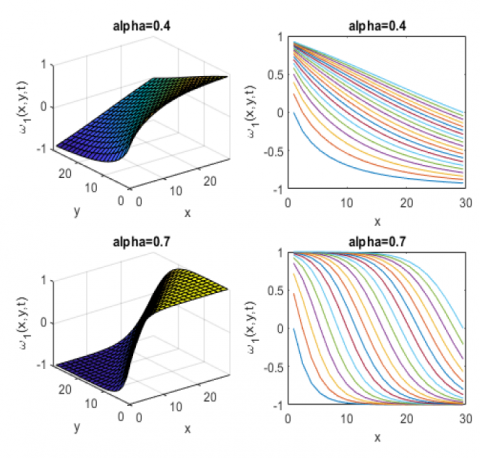
${{\omega }_{1}}=\pm \sqrt{-\frac{\beta }{\varepsilon }}+\frac{{{b}_{1}}}{2\xi }\left( -\eta -\eta \tanh \left( \frac{\eta \delta }{2} \right) \right),$ (38)
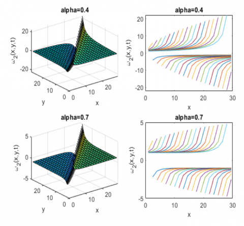
${{\omega }_{2}}=\pm \sqrt{-\frac{\beta }{\varepsilon }}+\frac{{{b}_{1}}}{2\xi }\left( -\eta -\eta \coth \left( \frac{\eta \delta }{2} \right) \right),$ (39)
${{\omega }_{3}}=\pm \sqrt{-\frac{\beta }{\varepsilon }}+\frac{{{b}_{1}}\left( -\eta -\eta \tanh \left( \eta \delta \right)\mp i\eta \operatorname{sech}\left( \eta \delta \right) \right)}{2\xi },$ (40)
${{\omega }_{4}}=\pm \sqrt{-\frac{\beta }{\varepsilon }}+\frac{{{b}_{1}}\left( -\eta -\eta \coth \left( \eta \delta \right)\mp \eta \operatorname{csch}\left( \eta \delta \right) \right)}{2\xi },$ (41)
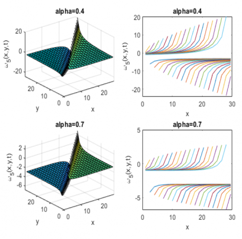
${{\omega }_{5}}=\pm \sqrt{-\frac{\beta }{\varepsilon }}+\frac{{{b}_{1}}}{4\xi }\left( -2\eta -\eta \tanh \left( \frac{\eta \delta }{4} \right)-\eta \coth \left( \frac{\eta \delta }{4} \right) \right),$ (42)
${{\omega }_{6}}=\pm \sqrt{-\frac{\beta }{\varepsilon }}+{{b}_{1}}\left( \frac{\eta \sqrt{{{Q}^{2}}+{{R}^{2}}}-\eta Q\cosh \left( \eta \delta \right)}{2\xi Q\sinh \left( \eta \delta \right)+2\xi R}-\frac{\eta }{2\xi } \right),$ (43)
${{\omega }_{7}}=\pm \sqrt{-\frac{\beta }{\varepsilon }}+{{b}_{1}}\left( \frac{-\eta \sqrt{{{R}^{2}}-{{Q}^{2}}}-\eta Q\sinh \left( \eta \delta \right)}{2\xi Q\cosh \left( \eta \delta \right)+2\xi R}-\frac{\eta }{2\xi } \right),$ (44)
where, Q and R are two non-zero real constant that satisfy ${{R}^{2}}-{{Q}^{2}}>0.$
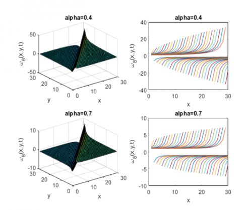
${{\omega }_{8}}=\pm \sqrt{-\frac{\beta }{\varepsilon }}+\frac{\pm {{b}_{1}}\eta {{e}^{\eta \delta }}}{\xi \mp \xi {{e}^{\eta \delta }}},$ (45)
${{\omega }_{9}}=\pm \sqrt{-\frac{\beta }{\varepsilon }}+\frac{\pm {{b}_{1}}\eta {{e}^{\eta \delta }}}{\xi i\mp \xi {{e}^{\eta \delta }}},$ (46)
${{\omega }_{10}}=\pm \sqrt{-\frac{\beta }{\varepsilon }}+{{b}_{1}}\frac{\eta \sqrt{{{Q}^{2}}-{{R}^{2}}}\pm \eta \left( Q{{e}^{\eta \delta }}-iR \right)}{\mp \xi Q\left( {{e}^{\eta \delta }}-{{e}^{-\eta \delta }} \right)\pm 2\xi iR},$ (47)
where, Q and R are two non-zero real constant that satisfy ${{Q}^{2}}-{{R}^{2}}>0.$
${{\omega }_{11}}=\pm \sqrt{-\frac{\beta }{\varepsilon }}+\frac{-{{b}_{1}}\eta \phi {{e}^{\eta \delta }}}{\xi +\xi \phi {{e}^{\eta \delta }}},$ (48)
${{\omega }_{12}}=\pm \sqrt{-\frac{\beta }{\varepsilon }}+\frac{-{{b}_{1}}\eta {{e}^{\eta \delta }}}{\xi \phi +\xi {{e}^{\eta \delta }}}\quad,$ (49)
where, ϕ is an arbitrary constant.
For η=0 and ξ≠0 and arbitrary constant ψ:
${{\omega }_{13}}=\pm \sqrt{-\frac{\beta }{\varepsilon }}+\frac{-{{b}_{1}}}{\xi \delta +\psi },$ (50)
where, $\delta =\frac{r{{x}^{\alpha }}}{\Gamma \left( \alpha +1 \right)}+\frac{s{{y}^{\alpha }}}{\Gamma \left( \alpha +1 \right)}\mp \frac{{{t}^{\alpha }}\sqrt{{{r}^{2}}{{\eta }^{2}}+{{s}^{2}}{{\eta }^{2}}-2\beta }}{\eta \Gamma \left( \alpha +1 \right)}.$
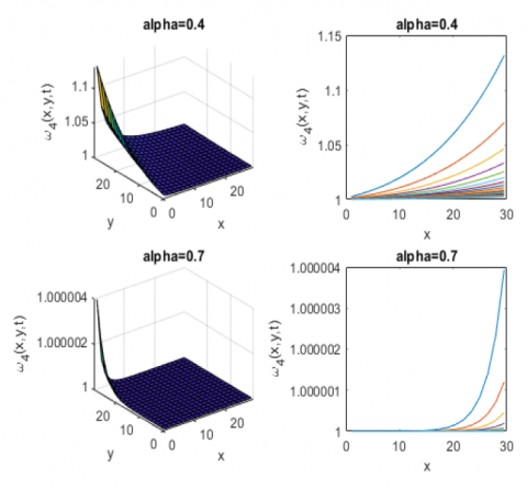
We have presented some physical graphs which are comparisons between α=0.4 and α=0.7. Figures 1, 2, 3 and 4 present the physical graphs of Eqns. (38), (39), (42) and (45) respectively when we set the parameters β=1, ε=-1, r=-1, s=1, η=1, ξ=1, t=100, 1≤x≤30, 1≤y≤30. We set:
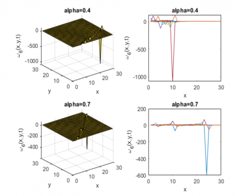
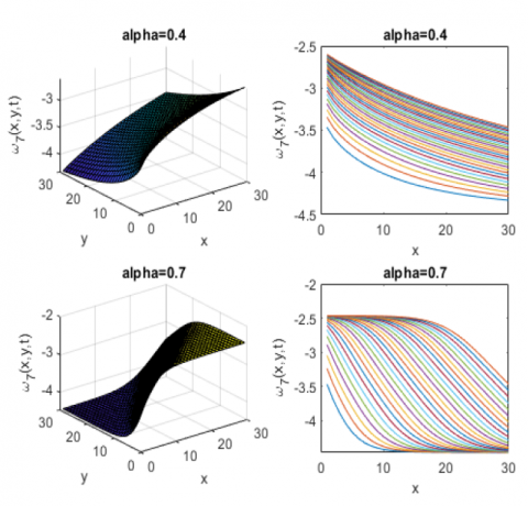
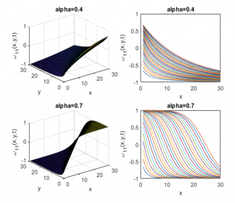
β=1, ε=-1, r=-1, s=1, η=1.2, ξ=1, t=100, 1≤x≤30, 1≤y≤30 in Eq. (41) which shown by Figure 5. When we substitute β=1, ε=-1, r=-1, s=1,η=1, ξ=1, t=100, Q=1, R=2, 1≤x≤30, 1≤y≤30 into Eqns. (43) and (44), the physical graphs are presented as Figures 6 and 7. Graphs of the physical wave are shown in Figures 8 and 9 when β=1, ε=-1, r=-1, s=1, η=1, ξ=1, t=100, ϕ=1, 1≤x≤30, 1≤y≤30 are substituted into Eqns. (48) and (49). Substituting β=1, ε=-1, r=-1, s=1, η=1, ξ=1, t=100, ψ=1, 1≤x≤30, 1≤y≤30 into Eq. (50), we get the physical graphs shown in Figure 10.
Figure 1. Kink wave of ω1
Figure 2. Solitary wave of ω2
Figure 3. Solitary wave of ω5
Figure 4. Solitary wave of ω8
Figure 5. Kink wave of ω4
Figure 6. Periodic wave of ω6
Figure 7. Kink wave of ω7
Figure 8. Kink wave of ω11
Figure 9. Kink wave of ω12
Figure 10. Periodic wave of ω13
3.2 The non-linear space and time fractional of (2+1)-dimensional GKP equation
Below are the exact results of traveling waves through the non-linear space and time fractional GKP equation:
$D_{x}^{\alpha }\left( D_{t}^{\alpha }\omega +6\omega D_{x}^{\alpha }\omega +6{{\omega }^{2}}D_{x}^{\alpha }\omega +D_{x}^{3\alpha }\omega \right)+D_{y}^{2\alpha }\omega =0,\,$ (51)
where, t>0, 0<α≤1 and ω=ω(x, y, t). Assuming that ω(x, y, t)=$\Theta$(δ) and using transformation in Eq. (24) again:
$r(-c{\Theta }'+6r\Theta {\Theta }'+6r{{\Theta }^{2}}{\Theta }'+{{r}^{3}}{\Theta }'''{)}'+{{s}^{2}}{\Theta }''=0.$ (52)
when, Eq. (52) is integrated twice with a constant of zero, the result is:
$-cr\Theta +3{{r}^{2}}{{\Theta }^{2}}+2{{r}^{2}}{{\Theta }^{3}}+{{r}^{4}}\frac{{{d}^{2}}\Theta }{d{{\delta }^{2}}}+{{s}^{2}}\Theta =0.$ (53)
After bringing Eq. (53) into balance, we found that K=1. As a result, Eq. (10) evolved into:
$\Theta \left( \delta \right)={{b}_{0}}+{{b}_{1}}G\left( \delta \right).$ (54)
Eq. (54) will be used in replacement of Eq. (53). In order to ensure that each coefficient was equivalent to zero, we first gathered up all of the words that belonged to the same power of G(δ) and then proceeded to do the following:
${{G}^{0}}\left( \delta \right)\,\,\,:\,\,\,-{{b}_{0}}cr+3b_{0}^{2}{{r}^{2}}+2b_{0}^{3}{{r}^{2}}+{{b}_{0}}{{s}^{2}}=0,$ (55)
${{G}^{1}}\left( \delta \right)\,\,\,:\,\,\,-{{b}_{1}}cr+6{{b}_{0}}{{b}_{1}}{{r}^{2}}+6b_{0}^{2}{{b}_{1}}{{r}^{2}}+{{b}_{1}}{{r}^{4}}{{\eta }^{2}}+{{b}_{1}}{{s}^{2}}=0,$ (56)
${{G}^{2}}\left( \delta \right)\,\,\,:\,\,\,3b_{1}^{2}{{r}^{2}}+6{{b}_{0}}b_{1}^{2}{{r}^{2}}+3{{b}_{1}}{{r}^{4}}\eta \xi =0,$ (57)
${{G}^{3}}\left( \delta \right)\,\,\,:\,\,2b_{1}^{3}{{r}^{2}}+2{{b}_{1}}{{r}^{4}}{{\xi }^{2}}=0.$ (58)
We reach the following result after calculating out the solution to the system of Eqns. (55)-(58):
${{b}_{0}}=\frac{-1\pm r\eta i}{2},$ (59)
${{b}_{1}}=\pm r\xi i,$ (60)
$c=\frac{{{s}^{2}}-2b_{0}^{2}{{r}^{2}}-{{r}^{4}}{{\eta }^{2}}}{r}.$ (61)
Eqns. (12)-(14), (26), and (59)-(61) give for the description of the different exact 13 solutions of the non-linear space and time fractional cKG equations. This generates all answers distinct from that presented in Eq (8).
For η, η2>0 and ξ≠0 these are real and not zero, then we get:
${{\omega }_{1}}=\frac{-1\pm r\eta i\pm ri\left( -\eta -\eta \tanh \left( \frac{\eta \delta }{2} \right) \right)}{2},$ (62)
${{\omega }_{2}}=\frac{-1\pm r\eta i\pm ri\left( -\eta -\eta \coth \left( \frac{\eta \delta }{2} \right) \right)}{2},$ (63)
${{\omega }_{3}}=\frac{-1\pm r\eta i\pm ri\left( -\eta -\eta \tanh \left( \eta \delta \right)\mp i\eta \operatorname{sech}\left( \eta \delta \right) \right)}{2},$ (64)
${{\omega }_{4}}=\frac{-1\pm r\eta i\pm ri\left( -\eta -\eta \coth \left( \eta \delta \right)\mp \eta \operatorname{csch}\left( \eta \delta \right) \right)}{2},$ (65)
${{\omega }_{5}}=\frac{-1\pm r\eta i}{2}\pm \frac{ri}{4}\left( -2\eta -\eta \tanh \left( \frac{\eta \delta }{4} \right)-\eta \coth \left( \frac{\eta \delta }{4} \right) \right),$ (66)
${{\omega }_{6}}=\frac{-1\pm r\eta i}{2}\pm ri\left( \frac{\eta \sqrt{{{Q}^{2}}+{{R}^{2}}}-\eta Q\cosh \left( \eta \delta \right)}{2Q\sinh \left( \eta \delta \right)+2R}-\frac{\eta }{2} \right),$ (67)
${{\omega }_{7}}=\frac{-1\pm r\eta i}{2}\pm ri\left( \frac{-\eta \sqrt{{{R}^{2}}-{{Q}^{2}}}-\eta Q\sinh \left( \eta \delta \right)}{2Q\cosh \left( \eta \delta \right)+2R}-\frac{\eta }{2} \right),$ (68)
where, Q and R are two non-zero real constant that satisfy ${{R}^{2}}-{{Q}^{2}}>0.$
${{\omega }_{8}}=\frac{-1\pm r\eta i}{2}\pm \frac{ri\eta {{e}^{\eta \delta }}}{1\mp {{e}^{\eta \delta }}},$ (69)
${{\omega }_{9}}=\frac{-1\pm r\eta i}{2}\pm \frac{ri\eta {{e}^{\eta \delta }}}{i\mp {{e}^{\eta \delta }}},$ (70)
${{\omega }_{10}}=\frac{-1\pm r\eta i}{2}\pm ri\left( \frac{\eta \sqrt{{{Q}^{2}}-{{R}^{2}}}\pm \eta \left( Q{{e}^{\eta \delta }}-iR \right)}{\mp Q\left( {{e}^{\eta \delta }}-{{e}^{-\eta \delta }} \right)\pm 2iR} \right),$ (71)
where, Q and R are two non-zero real constant that satisfy ${{Q}^{2}}-{{R}^{2}}>0.$
${{\omega }_{11}}=\frac{-1\pm r\eta i}{2}\mp \frac{ri\eta \phi {{e}^{\eta \delta }}}{1+\phi {{e}^{\eta \delta }}},$ (72)
${{\omega }_{12}}=\frac{-1\pm r\eta i}{2}\mp \frac{ri\eta {{e}^{\eta \delta }}}{\phi +{{e}^{\eta \delta }}},$ (73)
where, ϕ is an arbitrary constant.
For η=0 and ξ≠0 and arbitrary constant ψ, the solution to Eq. (10) is:
${{\omega }_{13}}=\frac{-1\pm r\eta i}{2}\mp \frac{r\xi i}{\xi \delta +\psi },$ (74)
where, $\delta =\frac{r{{x}^{\alpha }}}{\Gamma \left( \alpha +1 \right)}+\frac{s{{y}^{\alpha }}}{\Gamma \left( \alpha +1 \right)}\mp \frac{\left( {{s}^{2}}-2b_{0}^{2}{{r}^{2}}-{{r}^{4}}{{\eta }^{2}} \right){{t}^{\alpha }}}{r\Gamma \left( \alpha +1 \right)}.$
In this exploration, we were able to solve some non-linear fractional equations of crystal dislocation and internal waves on ocean shelf, known as the fractional cKG equation and the fractional GKP equation respectively. The exact solutions to the fractional cKG equation are offered in 13 different situations as Eqns. (38)-(50), which are more varied than the solutions obtained by the modified simple equation method [21]. Following the adjustment of a few parameters, some physical waves of these equations were found to be kink waves, solitary waves and periodic waves as seen in Figures 1-10. The exact solutions to the fractional GKP equation as seen in Eqns. (62)-(74) are complex solutions. There are 13 solutions total, which is one more than the number of solutions found using the (G'/G, 1/G)–Expansion method [26]. It can be shown that the generalized Bernoulli equation method is a highly successful way for solving non-linear fractional PDEs, and that this method will offer solutions to additional non-linear fractional equations.
[1] Alharbi, A.R., Almatrafi, M.B. (2020). Riccati-bernoulli Sub-ODE approach on the partial differential equations and applications. International Journal of Mathematics and Computer Science, 15(1): 367-388.
[2] Abdelrahman, M.A.E., Sohaly, M.A. (2018). The Riccati-bernoulli Sub-ODE technique for solving the deterministic (stochastic) generalized-zakharov system. International Journal of Mathematics and Systems Science, 1(3): 810. https://doi.org/10.24294/ijmss.v1i3.810
[3] Thadee, W., Chankaew, A., Phoosree, S. (2022). Effects of wave solutions on shallow-water equation, optical- fibre equation and electric-circuit equation. Maejo International Journal of Science and Technology, 16(3): 262-274.
[4] Akbar, M.A., Akinyemi, L., Yao, S., Jhangeer, A., Rezazadeh, H., Khater, M.M.A., Ahmad, H., Inc, M. (2021). Soliton solutions to the Boussinesq equation through sine-Gordon method and Kudryashov method. Results in Physics, 25: 104228. https://doi.org/10.1016/j.rinp.2021.104228
[5] Ilie, M., Biazar, J., Ayati, Z. (2018). The first integral method for solving some conformable fractional differential equations. Optical and Quantum Electronics, 50: 55. https://doi.org/10.1007/s11082-017-1307-x
[6] Hasan, F.L. (2020). First integral method for constructing new exact solutions of the important nonlinear evolution equations in physics. Journal of Physics: Conference Series, 1530: 012109. http://doi.org/10.1088/1742-6596/1530/1/012109
[7] Rahman, M.M., Habib, M.A., Ali, H.M.S., Miah, M.M. (2019). The generalized Kudryashov method: A renewed mechanism for performing exact solitary wave solutions of some NLEEs. Journal of Mechanics of Continua and Mathematical Sciences, 14(1): 323-339. https://doi.org/10.26782/jmcms.2019.02.00022
[8] Gaber, A.A., Aljohani, A.F., Ebaid, A., Machado, J.T. (2019). The generalized Kudryashov method for nonlinear space-time fractional partial differential equations of Burgers type. Nonlinear Dynamics, 95(1): 361-368. https://doi.org/10.1007/s11071-018-4568-4
[9] Kilicman, A., Silambarasan, R. (2018). Modified Kudryashov method to solve generalized Kuramoto-Sivashinsky equation. Symmetry, 10(10): 527. https://doi.org/10.3390/sym10100527
[10] Kumar, D., Seadawy, A.R., Joardar, A.K. (2018). Modified Kudryashov method via new exact solutions for some conformable fractional differential equations arising in mathematical biology. Chinese Journal of Physics, 56(1): 75-85. https://doi.org/10.1016/j.cjph.2017.11.020
[11] Babajanov, B., Abdikarimov, F. (2022). The application of the functional variable method for solving the loaded non-linear evaluation equations. Frontiers in Applied Mathematics and Statistics, 8: 912674. https://doi.org/10.3389/fams.2022.912674
[12] Rezazadeh, H., Vahidi, J., Zafar, A., Bekir, A. (2020). The functional variable method to find new exact solutions of the nonlinear evolution equations with dual-power-law nonlinearity. International Journal of Nonlinear Sciences and Numerical Simulation, 21(3-4): 249-257. https://doi.org/10.1515/ijnsns-2019-0064
[13] Baishya, C., Rangarajan, R. (2018). A new application of G′/G-expansion method for travelling wave solutions of fractional PDEs. International Journal of Applied Engineering Research, 13(11): 9936-9942. https://doi.org/10.37622/000000
[14] Phoosree, S., Chinviriyasit, S. (2021). New analytic solutions of some fourth-order nonlinear space-time fractional partial differential equations by G′/G-expansion method. Songklanakarin Journal of Science and Technology, 43(3): 795-801. https://doi.org/10.14456/sjst-psu.2021.105
[15] Mohyud-Din, S.T., Nawaz, T., Azhar, E., Akbar, M.A., (2017). Fractional sub-equation method to space-time fractional Calogero-Degasperis and potential Kadomtsev-Petviashvili equations. Journal of Taibah University for Science, 11(2): 258-263. https://doi.org/10.1016/j.jtusci.2014.11.010
[16] Yépez-Martínez, H., Gómez-Aguilar, J.F. (2019). Fractional sub-equation method for Hirota–Satsuma-coupled KdV equation and coupled mKdV equation using the Atangana’s conformable derivative. Waves in Random and Complex Media, 29(4): 678-693. https://doi.org/10.1080/17455030.2018.1464233
[17] Phoosree, S., Thadee, W. (2022). Wave effects of the fractional shallow water equation and the fractional optical fiber equation. Frontiers in Applied Mathematics and Statistics, 8: 900369. https://doi.org/10.3389/fams.2022.900369
[18] Sanjun, J., Chankaew, A. (2022). Wave solutions of the DMBBM equation and the cKG equation using the simple equation method. Frontiers in Applied Mathematics and Statistics, 8: 952668. https://doi.org/10.3389/fams.2022.95266
[19] Jumarie, G. (2006). Modified Riemann-Liouville derivative and fractional Taylor series of non-differentiable functions further results. Computers & Mathematics with Applications, 51(9-10): 1367-1376. https://doi.org/10.1016/j.camwa.2006.02.001
[20] Jumarie, G. (2009). Table of some basic fractional calculus formulae derived from a modified Riemann-Liouville derivative for non-differentiable functions. Applied Mathematics Letters, 22(3): 378-385. https://doi.org/10.1016/j.aml.2008.06.003
[21] Khan, K., Akbar, M.A. (2014). Exact solutions of the (2+1)-dimensional cubic Klein–Gordon equation and the (3+1)-dimensional Zakharov–Kuznetsov equation using the modified simple equation method. Journal of the Association of Arab Universities for Basic and Applied Sciences (2014) 15, 74-81. https://doi.org/10.1016/j.jaubas.2013.05.001
[22] Aslanova, G., Ahmetolan, S., Demirci, A. (2020). Nonlinear modulation of periodic waves in the cylindrical Gardner equation. Physical Review E, 102(5): 052215. https://doi.org/10.1103/PhysRevE.102.052215
[23] Liu, H., Yan, F. (2014). Bifurcation and exact travelling wave solutions for Gardner–KP equation. Applied Mathematics and Computation, 228(2014): 384-394. https://doi.org/10.1016/j.amc.2013.12.005
[24] Phoosree, S. (2019). Exact solutions for the estevez-mansfield-clarkson equation. Ph.D. dissertation. King Mongkut's University of Technology Thonburi, Thailand.
[25] Kolebaje, O.T., Popoola, O.O. (2014). Exact solution of fractional STO and jimbo-miwa equations with the generalized bernoulli equation method. The African Review of Physics, 9: 195-200.
[26] Shakeel, M., Mohyud-Din, S. T. (2014). Soliton solutions for the positive Gardner-KP equation by (G'/G, 1/G)–Expansion method. Ain Shams Engineering Journal, 5: 951-958. https://doi.org/10.1016/j.asej.2014.03.004