Tirupathi Maheshwaran![]() | Bapuji Pullepu*
| Bapuji Pullepu*![]() | Sandra Pinelas
| Sandra Pinelas![]()
© 2023 IIETA. This article is published by IIETA and is licensed under the CC BY 4.0 license (http://creativecommons.org/licenses/by/4.0/).
OPEN ACCESS
In this study, the Group Transformation method is employed to simulate the laminar free convection problem involving a viscous incompressible fluid on a vertically oriented cone with a uniform heat flux on its surface. The non-dimensional governing partial differential equations (PDEs) and their boundary conditions are reduced to ordinary differential equations (ODEs) with corresponding appropriate conditions. To solve the resulting non-linear ODEs, the Range-Kutta shooting method is applied. The temperature and velocity fields are graphically presented for various parameters, such as the semi-vertical angle and Prandtl number. Furthermore, the local Nusselt number and skin fraction are analyzed numerically.
group method, heat transfer, natural convection, ordinary differential equations, partial differential equations, vertical cone
Under the effect of gravitational force, the free convection flow was estimated most extensively as in most of the engineering and science applications as well as in nature, this phenomenon occurs more than other. When a fluid comes in contact with a heated surface, variations in temperatures results in buoyancy force, which furthers stimulates free convection. From the past few years, heat flux has been used widely in industrial applications, and also in the fields of engineering and technology. Heat Flux sensors are connected in control systems and are used for industrial measurement. Boiler fouling sensor (Fouling detection), flare monitoring and furnace monitoring, are a few examples of its application. Using heat flux can result in higher efficiency, better modelling and system safety. Many researchers have come up with a similarity solution for axisymmetric problem of laminar natural convection flow on a steady state vertical cone applying the Group Method transformation. For similarity analysis, Moran and Gaggioli [1] developed systematic group formalism. A quasi-linear hyperbolic second order PDE was analysed by Frydrychowicz and Singh [2] in their research to shows that conformal invariance of PDE’s under multi-parameter-dimensional group transformation implied the conformal in-variance of its characteristics. Heat transfer and fluid flow characteristics were studied by Abd-El-Malek and Badran [3] for unsteady and steady surfaces respectively, by analysing the free laminar convection on a circular vertical cylinder applying the Group Method. Another integral method was developed by Singh and Queeny [4] to treat the combination of heat and mass transfer in porous media by natural convection. One-parameter analysis was developed by Boutros et al. [5] for group transformation to Laplace equation in triangular domain. In this analysis the PDE transformation in polynomial form with boundary conditions, of any degree is reduced to ODE with its corresponding conditions. A general method was presented by Abd-El-Malek et al. [6] to apply group transformation with single parameter to multi-dimension diffusion equation. PDE with boundary condition is lowered to ODE with corresponding conditions by applying this transformation, and the problem is then solved by using the finite non-linear difference technique. Abd-El-Malek et al. [7] addressed the problem of drug diffusion via a thin membrane using a group theoretic method. Using group methods, in 2004 Abd-El-Malek et al. [8] analysed another efficient technique for unstable free-convection flow on a vertical plate, moving continuously. Ece [9] came up with similarity solutions for temperature and velocity profiles with boundary layer for determining the magnetic field effect on surface heat flux and skin friction. Their analysis was also applied to design a transformation for relating all solutions linked to the applied mixed thermal boundary conditions. The “magneto-elastico-viscous flow over a semi-infinite flat plate with heat transfer was studied using the group approach by Helal and Abd-El-Malek [10]. Kassem [11] developed a group theoretical technique which was used to present an unstable free convection flow from a vertical moving plate exposed to a constant heat flux. Under the coupled mass and heat diffusion, El-Kabeir et al. [12] investigated the thermal radiation effects on mass and heat transfer in hydro-magnetic natural convection flow across a vertical cone kept under uniform temperature of wall placed in a non-uniform porous media. For a convection chemical process, changing with time, a group similarity transformation method was developed by Kassem and Rashed [13]. Parmar and Timol [14] provided a deductive group approach for mass and heat transfer for a natural flow of non-Newtonian fluid immersed in porous material across a vertical cone. Abdul-Kahar and Kandasamy [15] applied the Lie group transformations to illustrate evolution of flow over a steady boundary layer, heat transmission, and nano-particle volume fraction across a porous stretch sheet and nano-fluid for varied values. Applying the deductive group method, Uddin et al. [16] developed new similarity transformation, as a result for free convection flow, the similarity solutions with heat transfer adjacent to flat moving plate placed horizontally with convective boundary condition. Parmar and Timol [17] developed a generic technique for solving the Rayleigh issue for an MHD Sisko fluid using a one-parameter general group transformation. Using a two-parameter group, Sojoudi et al. [18] established an efficient solution for free unstable convection, non-Newtonian fluid flow across a vertical plate moving continuously and exposed to heat flux constantly. For a magnetic nano fluid, the group analysis of its free convection flow with chemical reaction problem was by Uddin et al. [19]. Pranitha et al. [20] used the Lie scaling group transformation to investigate the effects of Soret, varying characteristics, and radiation on mixed convection flow over a vertical sheet inserted in porous material saturated with a power-law fluid. The controlling PDE and boundary conditions are lowered to ODE with acceptable boundary conditions, in this solution for natural steady laminar convection flow on an isothermal vertical cone was analysed by applying the group method approach designed by Immanuel et al. [21]. Kannan et al. [22] using group method approaches, investigated the influence of viscous dissipation on free convection steady flow from a non-isothermal vertical cone. Hossain and Paul [23] non-similarity and similarity solutions were designed by axisymmetric problems for natural convection flow on a steady state vertical cone. In 1992, Pop and Watanabe [24], and Lin [25] studied the flow on a vertical or cone frustum with non-uniform/uniform surface heat flux and non-porous/porous material. Further, the Control Layer Theory was also discussed in study [26]. Afify et al. [27] conducted a Lie group analysis for a power-law fluid over a stretched surface with MHD and also discussed many characteristics related to it. Morgan [28] came up with a theory which resulted in improvements in standard similarity techniques. To generate similarity solutions, Jain et al. [29] developed a group deductive method that works with group transformation approach. Rashad [30] used the Brinkman-Forchheimer-Darcy extended model for studying the natural convection flow on boundary layer around a sphere placed in a nano-fluid filled porous media. Garoosi et al. [31] discovered that lowering the size of the nano particles improves heat transfer rate and optimal particle loading (ϕopt). Makulati et al. [32] examined the natural convection of an alumina-water nanofluid in an inclined C-shaped enclosure in the presence of a magnetic field. Nia et al. [33] investigated the Natural Convection Heat Transfer of a Nanofluid in an L-Shape Enclosure with a Baffle. Numerical Study of MHD Nanofluid Natural Convection in a Baffled U-shaped Enclosure was created by Ma et al. [34]. Yang et al. [35] discovered CFD is used to quantitatively study the heat transfer enhancement and surface temperature non-uniformity improvement of spray cooling. The simulated results match the actual data well under verification conditions, with a maximum relative deviation of less than 7%, demonstrating the numerical reliability of the two-phase flow model based on the Euler-Lagrangian technique. The objective of the present work is to study the solution for group method of uniform surface heat flux from a vertical cone utilising laminar free convection, and the governing PDE and boundary conditions are reduced to an ODE with appropriate boundary conditions. The acquired differential equations are solved using the shooting technique, which has not received any attention in the literature. To ensure the accuracy of the numerical results, the current results are compared to those of Lin [25], Pop and Watanabe [24], which are shown to be in good agreement.
The present analysis, a consistent axisymmetric free convection of incompressible viscous flow is studied on a vertical cone having uniformly applied heat flux on its surface. It is assumed that viscous dissipation effects and pressure gradient along the boundary layer are negligible.
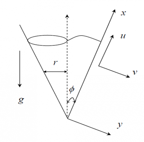
Figure 1. Physical model and co-ordinate system
The co-ordinate system is as shown in Figure 1, x signifying along the cone surface from the apex (x=0) and y signifying the distance normal to a cone surface. Temperature T'w on a cone surface is kept same, where temperature value is uniform, far from the temperature of cone surface. With the thermal buoyancy effect, an upward flow is created for T'w>T'∞. Other than the fluctuations in the densities in buoyancy force, where fluid properties are kept constant. For energy, momentum and continuity, their governing equations of boundary layer with Boussinesq approximations are as follows:
${{(ru)}_{x}}+{{(rv)}_{y}}=0\,$ (1)
$u{{u}_{x}}+v{{u}_{y}}=g\beta ({{T}^{'}}-{{T}^{'}}_{\infty })\cos \phi +\vartheta {{u}_{yy}}$ (2)
$u{{T}^{'}}_{x}+v{{T}^{'}}_{y}=\alpha {{T}^{'}}_{yy}$ (3)
The basic and restrictive conditions are as follows:
$\begin{align} & u(x,0)=\,v(x,0)=0,\,\,{{T}^{'}}_{y}=\frac{-{{q}_{w}}(x)}{k}\,\,\,\,\,\,at\,\,\,\,y=0 \\ & u(0,y)=0,\,\,{{T}^{'}}(0,\infty )={{T}_{\infty }}^{'}\,\,\,\,\,\,\,\,\,at\,\,\,\,x=0\,\, \\ & u(x,\infty )=0,\,\,\,\,{{T}^{'}}(x,\infty )=T\,\,\,\,\,\,\,at\,\,\,\,y\to \infty \\\end{align}$ (4)
Local Nusselt number Nux and Local skin friction τx are given by:
$\begin{align} & {{\tau }_{x}}=\mu {{\left( {{u}_{y}} \right)}_{y=0}}\,\,\,\,\,\, \\ & N{{u}_{x}}=\frac{x}{{{T}^{'}}_{w}-{{T}^{'}}_{\infty }}{{\left( -{{T}^{'}}_{y} \right)}_{y=0}} \\\end{align}$ (4a)
Utilization of enclosed dimensionless quantities:
$\begin{align} & {{x}^{*}}=\frac{x}{l},\,\,\,\,\,{{y}^{*}}=\frac{y}{l}\,{{({{G}_{{{r}_{l}}}})}^{\frac{1}{5}}},\,\,\,\,{{r}^{*}}=\frac{r}{l},\,\,\text{where}\,r=x\sin \varphi \\& {{u}^{*}}=\frac{ul}{\vartheta }{{({{G}_{{{r}_{l}}}})}^{\frac{-2}{5}}},\,\,\,\,{{v}^{*}}=\frac{vl}{\vartheta }{{({{G}_{{{r}_{l}}}})}^{\frac{-1}{5}}},\,\,\,\,T=\frac{({{T}^{'}}-{{T}^{'}}_{\infty }){{({{G}_{{{r}_{l}}}})}^{\frac{1}{5}}}}{ql/k}\, \\ & {{G}_{{{r}_{l}}}}=\frac{g\beta \,\,\,q\,{{l}^{4}}}{{{\vartheta }^{2}}k},\,\,\,\,\,\,\,\Pr =\frac{\vartheta }{\alpha } \\\end{align}$ (5)
Using (5), the reduction of Eqns. (1) to (3) yields the dimensionless form as follows:
${{({{r}^{*}}{{u}^{*}})}_{{{x}^{*}}}}+{{({{r}^{*}}{{v}^{*}})}_{{{y}^{*}}}}=0$ (6)
${{u}^{*}}{{u}^{*}}_{{{x}^{*}}}+{{v}^{*}}{{u}^{*}}_{{{y}^{*}}}=T\cos \phi +{{u}^{*}}_{{{y}^{*}}{{y}^{*}}}$ (7)
${{u}^{*}}{{T}_{{{x}^{*}}}}+{{v}^{*}}{{T}_{{{y}^{*}}}}=\frac{1}{\Pr }{{T}_{{{y}^{*}}{{y}^{*}}}}$ (8)
Given the following boundary conditions:
$\begin{align} & {{u}^{*}}({{x}^{*}},0)=0,\,\,\,\,\,{{v}^{*}}({{x}^{*}},0)=0,\,\,{{T}_{{{y}^{*}}}}=-1\,\,\,at\,\,\,{{y}^{*}}=0 \\ & {{u}^{*}}(0,{{y}^{*}})=0,\,\,\,\,\,T(0,{{y}^{*}})=0\,\,\,\,\,\,\,\,\,at\,\,\,\,{{x}^{*}}=0\, \\ & {{u}^{*}}({{x}^{*}},\infty )=0,\,\,\,\,\,T({{x}^{*}},\infty )=0\,\,\,\,as\,\,\,{{y}^{*}}\to \infty \\\end{align}$ (9)
From Eq. (4a), the local dimensionless local Nusselt number $N u_{x^*}$ and skin-friction $\tau_{x^*}$ becomes:
$\begin{align} & {{\tau }_{{{x}^{*}}}}=G{{r}_{l}}^{3/5}{{\left( {{u}^{*}}_{{{y}^{*}}} \right)}_{{{y}^{*}}=0}} \\ & N{{u}_{{{x}^{*}}}}=\frac{{{x}^{*}}G{{r}_{l}}^{1/5}}{{{T}_{{{y}^{*}}=0}}}{{\left( -{{T}_{{{y}^{*}}}} \right)}_{{{y}^{*}}=0}} \\\end{align}$ (9a)
Similarity variables are follows:
$\begin{align} & \omega ={{x}^{*}}{{r}^{*}}M({{x}^{*}},{{y}^{*}})\,\,\,\,\,\,\,\, \\ & T({{x}^{*}},{{y}^{*}})={{x}^{*}}\,\,T({{x}^{*}},{{y}^{*}}) \\\end{align}$ (9b)
In order to reduce the number of equations from 3 to 2, we introduce the stream function such that:
${{u}^{*}}=\frac{1}{{{r}^{*}}}{{\omega }_{{{y}^{*}}}}and\,\,{{v}^{*}}=\frac{-1}{{{r}^{*}}}{{\omega }_{{{x}^{*}}}}$ (9c)
Condition (6) is satisfied via a stream function, and (7) and (8) are switched to accompanying conditions.
${{\omega }_{{{y}^{*}}}}{{\left( \frac{1}{{{r}^{*}}}{{\omega }_{{{y}^{*}}}} \right)}_{{{x}^{*}}}}-\frac{1}{{{r}^{*}}}{{\omega }_{{{x}^{*}}}}{{\omega }_{{{y}^{*}}{{y}^{*}}}}=T{{r}^{*}}\cos \phi +{{\omega }_{{{y}^{*}}{{y}^{*}}{{y}^{*}}}}$ (10)
$\frac{1}{{{r}^{*}}}\left( {{\omega }_{{{y}^{*}}}}{{T}_{{{x}^{*}}}}-{{\omega }_{{{x}^{*}}}}{{T}_{{{y}^{*}}}} \right)=\frac{1}{\Pr }{{T}_{{{y}^{*}}{{y}^{*}}}}$ (11)
Boundary condition (9) communicated as:
$\begin{align} & \underset{{{y}^{*}}\to 0}{\mathop{\lim }}\,{{\omega }_{{{y}^{*}}}}=0\,\,\,\,\,\,\,\underset{{{y}^{*}}\to 0}{\mathop{\lim }}\,{{\omega }_{{{x}^{*}}}}=0\,\,\,\,\underset{{{y}^{*}}\to 0}{\mathop{\lim }}\,{{T}_{{{y}^{*}}}}=-1 \\ & \underset{{{y}^{*}}\to \infty }{\mathop{\lim }}\,{{\omega }_{{{y}^{*}}}}=0\,\,\,\,\,\,\underset{{{y}^{*}}\to \infty }{\mathop{\lim }}\,T=0 \\\end{align}$ (12)
Method of solution depend on the application of a one parameter group transformation to the PDE (10) to (11). Under this transformation the two independent variables will be reduced by one and the differential Eqns. (10) and (11) transform into ODE in only one independent variable, which is the similarity variable: $h: \bar{P}=C^p(b) P+k^p(b)$.
3.1 The group systematic formulation
The procedure is initiated with the group G, a class of one-parameter ‘b’ of the form:
$\left. \begin{align} & \overline{x}={{C}^{{{x}^{*}}}}(b){{x}^{*}}+{{k}^{{{x}^{*}}}}(b)\,\,\,\,\,\,\,\overline{y}={{C}^{{{y}^{*}}}}(b){{y}^{*}}+{{k}^{{{y}^{*}}}}(b) \\ & \overline{\omega }={{C}^{\omega }}(b)\omega +{{k}^{\omega }}(b)\,\,\,\,\,\,\,\,r={{C}^{{{r}^{*}}}}(b){{r}^{*}}+{{k}^{{{r}^{*}}}}(b) \\ & \overline{T}={{C}^{T}}(b)T+{{k}^{T}}(b) \\\end{align} \right\}$ (13)
$\left. \begin{align} & \overline{{{P}_{i}}}=\left( {}^{{{C}^{s}}}/{}_{{{C}^{i}}} \right){{P}_{i}} \\ & \overline{{{P}_{ij}}}=\left( {}^{{{C}^{s}}}/{}_{{{C}^{i}}{{C}^{j}}} \right){{P}_{ij}}\,\,\,\,\,\,\,\,\,\,\,\,\,\,\,\,\,\,\,\,\,\,\,\,\,\,\,\,i,\,\,\,j=x,y \\\end{align} \right\}\,$ (14)
3.2 Transformation
To transform the differential equation, transformation of derivatives is obtained from G via chain rule operations.
P stands for ω, r*, T.
Under the (13) and (14), Eqns. (10) and (11) are changed invariantly, becomes:
$\begin{align} & {{\overline{\omega }}_{y}}{{\left( \frac{1}{r}{{\overline{\omega }}_{y}} \right)}_{x}}-\frac{1}{r}{{\overline{\omega }}_{x}}{{\overline{\omega }}_{yy}}-r\overline{T}\overline{\cos \varphi }-{{\overline{\omega }}_{yyy}}= \\ & {{E}_{1}}(a)\left[ {{\omega }_{{{y}^{*}}}}{{\left( \frac{1}{{{r}^{*}}}{{\omega }_{{{y}^{*}}}} \right)}_{{{x}^{*}}}}-\frac{1}{{{r}^{*}}}{{\omega }_{{{x}^{*}}}}{{\omega }_{{{y}^{*}}{{y}^{*}}}}-{{r}^{*}}T\cos \varphi -{{\omega }_{{{y}^{*}}{{y}^{*}}{{y}^{*}}}} \right]\, \\\end{align}$ (15)
$\begin{align} & \frac{1}{r}\left[ {{\overline{\omega }}_{y}}{{\overline{T}}_{x}}-{{\overline{\omega }}_{x}}{{\overline{T}}_{y}} \right]-\frac{1}{\Pr }{{\overline{T}}_{yy}} \\ & ={{E}_{2}}(a)\left[ \frac{1}{{{r}^{*}}}\left( {{\omega }_{{{y}^{*}}}}{{T}_{{{x}^{*}}}}-{{\omega }_{{{x}^{*}}}}{{T}_{{{y}^{*}}}} \right)-\frac{1}{\Pr }{{T}_{{{y}^{*}}{{y}^{*}}}} \right]\,\, \\\end{align}$ (16)
where, E1(a), E2(a) are functions or Constant.
$\begin{align} & \frac{{{C}^{\omega }}{{C}^{T}}}{{{C}^{{{r}^{*}}}}{{C}^{{{x}^{*}}}}{{C}^{{{y}^{*}}}}}\left[ \frac{1}{{{r}^{*}}}{{\omega }_{{{y}^{*}}}}{{\omega }_{{{x}^{*}}{{y}^{*}}}}-\frac{1}{{{r}^{*}}^{2}}{{\left( {{\omega }_{{{y}^{*}}}} \right)}^{2}}{{r}^{*}}_{{{x}^{*}}}-\frac{1}{{{r}^{*}}}{{\omega }_{{{y}^{*}}{{y}^{*}}}} \right] \\ & -{{r}^{*}}{{C}^{{{r}^{*}}}}{{C}^{T}}T\cos \phi -\frac{{{C}^{\omega }}}{{{({{C}^{{{y}^{*}}}})}^{2}}}{{\omega }_{{{y}^{*}}{{y}^{*}}{{y}^{*}}}}+{{A}_{1}}(a) \\ & ={{V}_{1}}(a)\left[ {{\omega }_{{{y}^{*}}}}{{\left( \frac{1}{{{r}^{*}}}{{\omega }_{{{y}^{*}}}} \right)}_{{{x}^{*}}}}-\frac{1}{{{r}^{*}}}{{\omega }_{{{x}^{*}}}}{{\omega }_{{{y}^{*}}{{y}^{*}}}}-T{{r}^{*}}\cos \phi -{{\omega }_{{{y}^{*}}{{y}^{*}}{{y}^{*}}}} \right] \\\end{align}$ (17)
$\begin{align} & \frac{{{C}^{\omega }}{{C}^{T}}}{{{C}^{{{r}^{*}}}}{{C}^{x}}{{C}^{y}}}\frac{1}{{{r}^{*}}}\left( {{\omega }_{{{y}^{*}}}}{{T}_{{{x}^{*}}}}-{{\omega }_{{{x}^{*}}}}{{T}_{{{y}^{*}}}} \right)-\frac{1}{\Pr }\frac{{{C}^{T}}}{{{({{C}^{{{y}^{*}}}})}^{2}}}{{T}_{{{y}^{*}}{{y}^{*}}}}+{{A}_{2}}(a) \\& ={{V}_{2}}(a)\left[ \frac{1}{{{r}^{*}}}\left( {{\omega }_{{{y}^{*}}}}{{T}_{{{x}^{*}}}}-{{\omega }_{{{x}^{*}}}}{{T}_{{{y}^{*}}}} \right)-\frac{1}{\Pr }{{T}_{{{y}^{*}}{{y}^{*}}}} \right] \\\end{align}$ (18)
where,
$\begin{aligned} & \mathrm{A}_1(a)=\sum_{n=1}^{\infty}\left(\begin{array}{c}-1 \\ n\end{array}\right)\left(\frac{k^{r^*}}{C^{r^*} r^*}\right)^m \frac{\left(C^\omega\right)^2}{C^{r^*} C^{x^*}\left(C^{y^*}\right)^2} \frac{1}{r^*}\left(\omega_{y^*} \omega_{x^* y^*}-\omega_{x^*} \omega_{y^* y^*}\right) \\ & -\sum_{n=1}^{\infty}(-2)\left(\frac{k^{r^*}}{C^{r^*} r^*}\right)^m \frac{\left(C^\omega\right)^2}{C^{r^*} C^{x^*}\left(C^{y^*}\right)^2} \frac{1}{r^{* 2}}\left(\omega_{y^*}\right)^2 r_{x^*}^* \\
& -\left(C^* k^{r^*} r^*+k^{r^*} C^{r^*} T\right)\left(C^{\cos \phi} \cos \phi+k^{\cos \phi}\right)\end{aligned}$ (19)
$\begin{aligned} & A_2(a)=\sum_{n=1}^{\infty}\left(\begin{array}{l}-1 \\ n\end{array}\right)\left(\frac{k^{r^*}}{C^{r^*} r^*}\right)^n \\ & \frac{C^\omega C^T}{C^{r^*} C^{x^*} C^{y^*}} \frac{1}{r^*}\left(\omega_{y^*} T_{x^*}-\omega_{x^*} T_{y^*}\right)\end{aligned}$ (20)
Invariance of Eqns. (17) and (18) $\Rightarrow A_1(b)=0=A_2(b)$.
By substituting, the above equations are satisfied.
${{k}^{{{r}^{*}}}}={{k}^{T}}={{k}^{{{y}^{*}}}}=0$ (21)
$\frac{{{({{C}^{\omega }})}^{2}}}{{{C}^{{{r}^{*}}}}{{C}^{{{x}^{*}}}}{{({{C}^{{{y}^{*}}}})}^{2}}}=\frac{{{C}^{\omega }}}{{{\left( {{C}^{{{y}^{*}}}} \right)}^{3}}}=\frac{{{C}^{\omega }}}{{{C}^{{{y}^{*}}}}}={{C}^{{{r}^{*}}}}{{C}^{T}}={{V}_{1}}(b)$ (22)
$\frac{{{C}^{\omega }}{{C}^{T}}}{{{C}^{{{r}^{*}}}}{{C}^{{{x}^{*}}}}{{C}^{{{y}^{*}}}}}=\frac{{{C}^{T}}}{{{\left( {{C}^{{{y}^{*}}}} \right)}^{2}}}={{V}_{2}}(b)$ (23)
These yields:
${{C}^{{{x}^{*}}}}={{\left( {{C}^{{{y}^{*}}}} \right)}^{2}},\,\,\,{{C}^{{{r}^{*}}}}=\frac{1}{{{\left( {{C}^{{{y}^{*}}}} \right)}^{2}}},\,\,\,\,{{C}^{\omega }}={{C}^{{{y}^{*}}}}$ (24)
Boundary Eqns. (19) and (20) are also invariant:
${{k}^{{{r}^{*}}}}={{k}^{T}}=0,\,\,\,\,\,\,{{C}^{T}}=1\,$ (25)
Finally, a limited, exhaustive G that is constantly changing, (17) and (18) conditions and the most extreme conditions (19) and (20) We get G from the above conditions.
$G=\left\{ \begin{align} & \overline{x}={{({{C}^{y}})}^{2}}{{x}^{*}}+{{k}^{{{x}^{*}}}} \\ & \overline{y}={{C}^{{{y}^{*}}}}{{y}^{*}} \\ & r=\frac{{{r}^{*}}}{{{\left( {{C}^{{{y}^{*}}}} \right)}^{2}}} \\ & \overline{\omega }={{C}^{{{y}^{*}}}}\omega +{{k}^{\omega }} \\ & \overline{T}=T \\\end{align} \right.$ (26)
3.3 Group transformation of the boundary layer flow equations
Our aim is to make use of group methods ro represent the problem in the form of an ODE in a single independent variable. Then we have to proceed in our analysis to obtain a complete set of absolute invariants.
If $v=v\left(x^*, y^*\right)$ is the absolute invariants of the independent variables x* and y*, then:
${{m}_{j}}({{x}^{*}},{{y}^{*}},\,\omega ,\,\,\phi ,{{r}^{*}},T)={{M}_{j}}(\upsilon ({{x}^{*}},{{y}^{*}}))\,\,\,\,j=1,2,3$ (27)
In group theory, using central assumptions is that if function mj (x*, y*, ω, ϕ, r*, T) satisfies the even derivative state of the first prompt, then one parameter group is levelled and unchanging. It states that:
$\begin{array}{ll}\sum_{i=1}^5\left(\chi_i w_i+\delta_i\right) \frac{\partial m}{\partial w_i}=0, & w_i=x^*, y^*, \omega, r^*, T \\ \text { where } \quad \chi_i=\frac{\partial C^{w_i}}{\partial b}(b) & \delta_i=\frac{\partial k^{w_i}}{\partial b}\left(b^0\right)\end{array}$ (28)
Since $k^{r^*}=k^T=k^{y^*}=0$.
From Eq. (23) and using (22) we get:
$\begin{aligned} & \delta_2=\frac{\partial k^y}{\partial b}\left(b^0\right)=0, \delta_4=\frac{\partial k^{r^*}}{\partial b}\left(b^0\right)=0, \delta_5=\frac{\partial k^T}{\partial b}\left(b^0\right)=0 \\ & \delta_3=\frac{\partial k^\omega}{\partial b}\left(b^0\right)=0 \quad \text { (ie) } \delta_2=\delta_3=\delta_4=\delta_5=0\end{aligned}$
By satisfies the first order linear PDE, υ(x*, y*) is an invariant by Eq. (22):
$({{\chi }_{1}}{{x}^{*}}+{{\delta }_{1}})\frac{\partial \upsilon }{\partial {{x}^{*}}}+{{\chi }_{2}}{{y}^{*}}\frac{\partial \upsilon }{\partial {{y}^{*}}}=0\,$ (29)
From the above equation we get:
$\frac{\partial \upsilon }{\partial {{x}^{*}}}=0$ (30)
Therefore equation:
$\upsilon ={{y}^{*}}$ (31)
Similarly, not changing the analysis of ω, r*, T dependent variables:
$\begin{gathered}\omega\left(x^*, y^*\right)=\Gamma_1\left(\mathrm{x}^*\right) \mathrm{M}(\iota), \\ r^*\left(x^*, y^*\right)=\Gamma_2\left(\mathrm{x}^*\right) \mathrm{E}(\iota), \\ T\left(x^*, y^*\right)=\mathrm{T}(v)\end{gathered}$ (32)
where, $\Gamma_1\left(\mathrm{x}^*\right), \Gamma_2\left(\mathrm{x}^*\right), \mathrm{M}(\iota), \& \mathrm{E}(\iota)$ are functions that are computed. Since r*(x*, y*) is independent of y*:
${{r}^{*}}({{x}^{*}},{{y}^{*}})={{r}^{*}}_{0}$ (33)
As the general analysis proceeds, the established form of the dependent and independent absolute invariant is used to obtain ODEs. Generally, the absolute invariant υ(x*, y*) has the form given in condition (31).
Substitute Eq. (32) into Eq. (17) and after dividing Г1(x*), we get:
$\begin{aligned} & (17) \Rightarrow \frac{1}{r^*} \omega_{y^*} \omega_{x^* y^*}-\frac{1}{r^{* 2}}\left(\omega_{y^*}\right)^2 r_{x^*}^*-\frac{1}{r^*} \omega_{x^*} \omega_{y^* y^*} -T r^* \cos \phi-\omega_{y^* y^* y^*}=0\end{aligned}$ $\begin{aligned} & M^{\prime \prime \prime}+\frac{1}{r_0^* \Gamma_2} M M^{\prime \prime} \frac{\partial \Gamma_1}{\partial x^*}-\left(\frac{1}{r_0^* \Gamma_2} \frac{\partial \Gamma_1}{\partial x^*}-\frac{\Gamma_1}{r_0^* \Gamma_2^2} \frac{\partial \Gamma_2}{\partial x^*}\right) M^{\prime 2} +\frac{r_0^* \Gamma_2 \Gamma_3}{\Gamma_1} T \cos \phi=0\end{aligned}$ (34)
If we substitute the conditions (26) to (28) into condition (13), we get:
$\begin{aligned} & \frac{1}{r^*}\left(\omega_{y^*} T_{x^*}-\omega_{x^*} T_{y^*}\right)-\frac{1}{\operatorname{Pr}} T_{y^* y^*}=0 \\ & \frac{1}{r^*{ }_0 \Gamma_2} \frac{\partial \Gamma_1}{\partial x^*} M(v) \frac{d T}{d y^*}+\frac{1}{\operatorname{Pr}} \frac{d^2 T}{d y^{* 2}}=0\end{aligned}$ (35)
${{C}_{1}}=\frac{1}{{{r}^{*}}_{0}{{\Gamma }_{2}}}\frac{\partial {{\Gamma }_{1}}}{\partial {{x}^{*}}},\,\,\,\,\,{{C}_{2}}=\frac{{{\Gamma }_{1}}}{{{r}^{*}}_{0}{{\Gamma }_{2}}^{2}}\frac{\partial {{\Gamma }_{2}}}{\partial {{x}^{*}}},\,\,\,\,\,{{C}_{3}}=\frac{{{r}^{*}}_{0}{{\Gamma }_{2}}{{\Gamma }_{3}}}{{{\Gamma }_{1}}}$ (36)
The above are random coefficients.
By utilizing above documentations of condition (36), the conditions (34) and (35) lessens to:
${{M}^{'''}}+{{C}_{1}}M\,{{M}^{''}}-({{C}_{1}}-{{C}_{2}}){{M}^{{{'}^{2}}}}+{{C}_{3}}\cos \phi T=0$ (37)
${{C}_{1}}M\,\frac{dT}{d{{y}^{*}}}+\frac{1}{\Pr }\frac{{{d}^{2}}T}{d{{y}^{*}}^{2}}=0$ (38)
There are corresponding boundary conditions.
${{M}^{'}}(0)=0,\,\,\,\,\,\,\frac{dT}{d{{y}^{*}}}\left( 0 \right)=-1,\,\,{{M}^{'}}(\infty )=T(\infty )=0$ (39)
Case (i) use values, ${{C}_{1}}=\frac{3}{4},\,\,\,\,\,{{C}_{2}}=\frac{1}{4}\,\,\,\,\And {{C}_{3}}=1$ in Eqns. (37) and (38) we get:
${{M}^{'''}}+\frac{3}{4}M\,{{M}^{''}}-\frac{1}{2}{{M}^{{{'}^{2}}}}+\cos \phi T=0$ (40)
$\frac{3}{4}M\,\frac{dT}{d{{y}^{*}}}+\frac{1}{\Pr }\frac{{{d}^{2}}T}{d{{y}^{*}}^{2}}=0\,\,\,\,\,(or)\frac{{{d}^{2}}T}{d{{y}^{*}}^{2}}+\frac{3}{4}\Pr M\,\frac{dT}{d{{y}^{*}}}=0$ (41)
Case (ii) put ${{C}_{1}}=\frac{7}{4},\,\,\,\,\,{{C}_{2}}=\frac{5}{4}\,\,\,\,\And {{C}_{3}}=1$ in Eqns. (37) and (38) we obtain:
${{M}^{'''}}+\frac{7}{4}M\,{{M}^{''}}-\frac{1}{2}{{M}^{{{'}^{2}}}}+\cos \phi T=0$ (42)
$\frac{7}{4}M\,\frac{dT}{d{{y}^{*}}}+\frac{1}{\Pr }\frac{{{d}^{2}}T}{d{{y}^{*}}^{2}}=0\,\,\,\,\,(or)\frac{{{d}^{2}}T}{d{{y}^{*}}^{2}}+\frac{7}{4}\Pr M\,\frac{dT}{d{{y}^{*}}}=0$ (43)
With boundary conditions:
${{M}^{'}}(0)=0,\,\,\,\,\,\,\,\,\,\frac{dT}{d{{y}^{*}}}\left( 0 \right)=-1,\,\,\,\,\,{{M}^{'}}(\infty )=T(\infty )=0\,$ (44)
Using Eqns. 9(b) and 9(c) into Eq. 9(a), the local dimensionless Nusselt number and skin friction becomes:
${{\tau }_{{{x}^{*}}}}G{{r}_{l}}^{-3/5}={{x}^{*}}{{M}^{''}}(0\,),\,\,\,\,\,N{{u}_{{{x}^{*}}}}G{{r}_{l}}^{-1/5}=-{{x}^{*}}\frac{{{T}^{'}}(0\,)}{T(0)}$
Eqns. (40) to (43) with boundary conditions (44) were solved by numerically using the fourth-order R-K method. The velocity and temperature profiles of the cone for Pr=0.72 are displayed in Figure 2 and the numerical values of local skin-friction $\tau_x^*$, temperature T, for different values of prandtl number are shown in Table1 are compared with similarity solution of Lin [25] using suitable transformation. It is observed that the results are in good agreement with each other. It is also noticed that the present result agrees well with those of Lin [25] and Pop and Watanabe [24] (as pointed out in Table 1).
Table 1. Skin-friction and temperature values are Comparison with Lin [25]
|
|
Local skin friction |
Temperature |
||||
|
|
Lin result [25] |
Present result |
Lin result [25] |
Present result |
||
|
Pr |
M’’(0) |
(7/4) M’’(0) |
$\tau_x^*$ |
-T(0) |
-(7/4) T(0) |
T |
|
0.72 |
0.87830 |
1.2250 |
1.2154 |
1.53213 |
1.7896 |
1.7783 |
|
1 |
0.78336 |
1.0799 |
1.0735 |
1.39071 |
1.6324 |
1.6272 |
|
2 |
0.59251 |
0.8303 |
0.8295 |
1.16102 |
1.3532 |
1.3576 |
|
4 |
0.46507 |
0.6573 |
0.6330 |
0.97802 |
1.1490 |
1.1501 |
|
6 |
0.39700 |
0.5562 |
0.5499 |
0.88910 |
1.0501 |
1.0402 |
|
8 |
0.34963 |
0.4905 |
0.4849 |
0.83251 |
0.9806 |
0.9764 |
|
10 |
0.32645 |
0.4495 |
0.4459 |
0.78910 |
0.9291 |
0.9280 |
|
100 |
0.13071 |
0.1839 |
0.1812 |
0.49013 |
0.5572 |
0.5404 |
Figure 2. Velocity and temperature profiles comparison
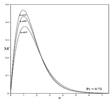
Figure 3. Different values of f on velocity profiles
Figure 4. Different values of f on temperature profiles
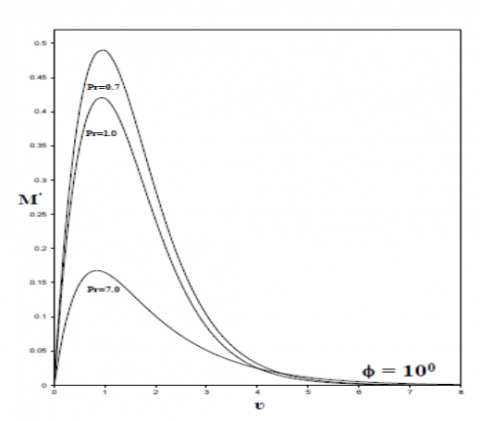
Figure 5. Different Pr. values on velocity profiles
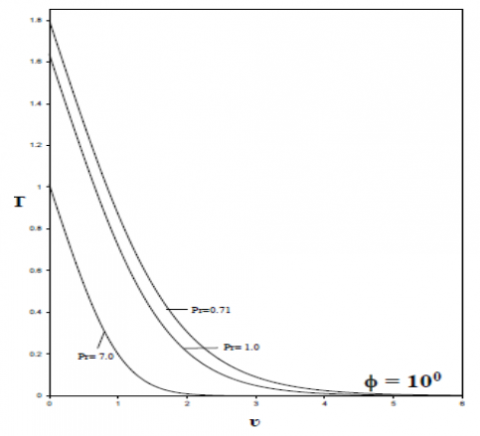
Figure 6. Different Pr. values on temperature profiles
Temperate and Velocity profile of a cone for Pr=0.72 is graphically represented in Figure 2. The temperature and velocity profiles shown in Figures 3-6 with different $\phi$ and Pr parameters. For Pr=0.71, and varying values of $\phi$, the velocity profile is shown in Figure 3. As f increases near a cone’s apex, the momentum force on a cone surface decreases. Therefore, differences in steady state and temporal maximum velocity value lowers as $\phi$ values of a cone (semi-vertical angle) increase. Also, with decreasing velocity, $\phi$ rises. The boundary layer momentum becomes thick; hence it increases the time required to acquire a steady state for rising value of $\phi$. For Pr =0.71, and varying values of $\phi$, temperature profiles are given in Figure 4. Further thickness and temperature of boundary layer also increases.
At ϕ=10°, different Pr values, the temperature and velocity profiles are represented in Figures 5 and 6. Viscosity increases and thermal conductivity decreases, when Pr increases. From the figure, it can be concluded that with higher Pr, variations in the maximum and steady-state value over time decreased and local skin-friction and Nusselt number profiles are against the $\phi$ angle of a cone for different Pr values.
The group technique was used to present numerical solutions of steady laminar free convection on a vertical cone with a uniform heat flux imposed on a surface. Using R-K method, the dimensionless boundary layer equation is solved. Following conclusions were made:
·If the parameters $\phi$ and Pr are increased, the velocity will decrease.
·The temperature rises and decreasing Pr with increasing fvalue.
·Increasing $\phi$, increases the impulse boundary layer.
·Decreasing $\phi$ and increasing Pr, thins the thermal boundary layer.
·The cause of $\phi$ on local Nusselt number $N u_{x^*}$ and local skin friction $\tau_{x^*}$ is low approximately equal to the cone’s apex and slowly increases as the distance from apex increases.
·When Pr or fvalue is reduced, local skin-frictions increases.
·Effect of Increasing $\phi$ or decreasing Pr, local Nusselt numbers reduce.
[1] Moran, M.J., Gaggioli, R.A. (1968). A new systematic formulation for similarity analysis with application to boundary–Layer flows. U.S. Army math. Research centre, Tech, Summary Report No.918,
[2] Frydrychowicz, W., Singh, M.C. (1986). Group theoretic and similarity analysis of hyperbolic partial differential equations. Journal of Mathematical Analysis and Applications, 114(1): 75-99. http://dx.doi.org/10.1016/0022-247X(86)90067-3
[3] Abd-El-Malek, M.B., Badran, N.A. (1990). Group method analysis of unsteady free-convective laminar boundary-layer flow on a nonisothermal vertical circular cylinder. Acta Mechanica, 85: 193-206. https://doi.org/10.1007/BF01181517
[4] Singh, P., Queeny. (1997). Free convection heat and mass transfer along a vertical surface in a porous medium. Acta Mechanica, 123(1-4): 69-73. https://doi.org/10.1007/BF01178401
[5] Boutros, Y.Z., Abd-El-Malek, M.B., El-Awadi, I.A., El-mansi, S.M.A. (1997). Group method analysis of the potential equation in triangular regions. Symmetry in Nonlinear Mathematical Physics, 2: 418-428.
[6] Abd-El-Malek, M.B., Badran, N.A., Hassan, H.S. (2002). Using group theoretic method to solve multi-dimensional diffusion equation. Journal of Computational and Applied Mathematics, 147(2): 385-395. https://doi.org/10.1016/S0377-0427(02)00474-0
[7] Abd-El-Malek, M.B., Kassem, M.M., Meky, M.L. (2002). Group theoretic approach for solving the problem of diffusion of a drug through a thin membrane. Journal of Computational and Applied Mathematics, 140(1-2): 1-11. https://doi.org/10.1016/S0377-0427(01)00516-7
[8] Abd-El-Malek, M.B., Kassem, M.M., Mekky, M.L. (2004). Similarity solutions for unsteady free-convection flow from a continuous moving vertical surface. Journal of Computational and Applied Mathematics, 164: 11-24. https://doi.org/10.1016/S0377-0427
[9] Ece, M.C. (2005). Free convection flow about a cone under mixed thermal boundary conditions and a magnetic field. Applied Mathematical Modelling, 29(11): 1121-1134. https://doi.org/10.1016/j.aprh.2005
[10] Helal, M.M., Abd-El-Malek, M.B. (2005). Group method analysis of magneto-elastico-viscous flow along a semi-infinite flat plate with heat transfer. Journal of Computational and Applied Mathematics, 173(2): 199-210. https://doi.org/10.1016/j.cam.2004.03.007
[11] Kassem, M. (2006). Group solution for unsteady free-convection flow from a vertical moving plate subjected to constant heat flux. Journal of Computational and Applied Mathematics, 187(1): 72-86. https://doi.org/10.1016/j.cam.2005.03.037
[12] El-Kabeir, S.M.M., El-Hakiem, M.A., Rashad, A.M. (2007). Group method analysis for the effect of radiation on MHD coupled heat and mass transfer natural convection flow water vapor over a vertical cone through porous medium. International Journal of Applied Mathematics and Mechanics, 3(2): 35-53.
[13] Kassem, M.M., Rashed, A.S. (2008). Group similarity transformation of a time dependent chemical convective process. International Journal of Mathematical and Computational Sciences, 2(4): 249-256. https://scholar.waset.org/1999.7/286
[14] Parmar, H., Timol, M.G. (2011). Deductive group technique for MHD coupled heat and mass transfer natural convection flow of non-Newtonian power law fluid over a vertical cone through porous medium. International Journal of Applied Mathematics and Mechanics, 7(2): 35-50.
[15] Abdul-Kahar, R., Kandasamy, R. (2011). Scaling group transformation for boundary-layer flow of a nanofluid past a porous vertical stretching surface in the presence of chemical reaction with heat radiation. Computers & Fluids, 52: 15-21. https://doi.org/10.1016/j.compfluid.2011.08.003
[16] Uddin, M.J., Khan, W.A., Ismail, A.I., Hamad, M.A.A. (2015). New similarity solution of boundary layer flow along a continuously moving convectively heated horizontal plate by deductive group method. Thermal Science, 19(3): 1017-1024. https://doi.org/10.2298/TSCI130115014U
[17] Parmar, H., Timol, M.G. (2014). Group theoretic analysis of Rayleigh problem for a non-Newtonian MHD Sisko fluid past semi infinite plate. International Journal of Advance Applied Maths and Mech., 1(3): 96-108,
[18] Sojoudi, A., Mazloomi, A., Saha, S.C., Gu, Y.T. (2014). Similarity solution flow and heat transfer of non-Newtonian fluid over a stretching surface. Journal of Applied Mathematics, 2014: 718319. https://doi.org/10.1155/2014/718319
[19] Uddin, M., Bég, O.A., Aziz, A., Ismail, A.I. (2015). Group analysis of free convection flow of a magnetic nanofluid with chemical reaction. Mathematical Problems in Engineering, 2015: 621503. https://doi.org/10.1155/2015/621503
[20] Pranitha, J., Suman, G.V., Srinivasacharya, D. (2017). Scaling group transformation for mixed convection in a power-law fluid saturated porous medium with effects of soret, radiation and variable properties. Frontiers in Heat and Mass Transfer, 9: 39. https://doi:10.5098/hmt.9.39
[21] Immanuel, Y., Pullepu, B., Maheshwaran, T. (2019, June). Group method study of steady laminar natural convection flow past an isothermal vertical cone. In AIP Conference Proceedings, 2112(1): 020064. https://doi.org/10.1063/1.5112249
[22] Kannan, R.M., Pullepu, B., Sambath, P. (2019). Group solution for free convection flow of dissipative fluid from non-isothermal vertical cone. In AIP Conference Proceedings, 2112(1): 020014. https://doi.org/10.1063/1.5112199
[23] Hossain, M.A., Paul, S.C. (2001). Free convection from a vertical permeable circular cone with non-uniform surface heat flux. Heat and Mass Transfer, 37(2-3): 167-173. https://doi.org/10.1007/s002310000129
[24] Pop, I., Watanabe, T. (1992). Free convection with uniform suction or injection from a vertical cone for constant wall heat flux. International Communications in Heat and Mass Transfer, 19: 275-283. https://doi.org/10.1016/0735-1933(92)90038-J
[25] Lin, F.N. (1976). Laminar free convection from a vertical cone with uniform surface heat flux. Letters Heat Mass Transfer, 3: 49-58. https://doi.org/10.1016/0094-4548(76)90041-2
[26] Schlichting, H. (1979). Boundary Layer Theory. 7th Ed., Mc Graw-Hill, New York, USA.
[27] Afify, A.A., Uddin, M.J., Ferdows, M. (2014). Scaling group transformation for MHD boundary layer flow over permeable stretching sheet in presence of slip flow with Newtonian heating effects. Applied Mathematics and Mechanics, 35: 1375-1386. https://doi.org/10.1007/S10483-014-1873-7
[28] Morgan, A.J.A. (1952). The reduction by one of the number of independent variables in some systems of partial differential equations. The Quarterly Journal of Mathematics, 3(1): 250-259. https://doi.org/10.1093/qmath/3.1.250
[29] Jain, N., Darji, R.M., Timol, M.G. (2014). Similarity solution of natural convection boundary layer flow of non-Newtonian Sutterby fluids. International Journal of Advanced Applied Mathematical Research, 2(2): 150-158.
[30] Rashad, A.M. (2014). Natural convection boundary layer flow along a sphere embedded in a porous medium filled with a nanofluid. Latin American Applied Research, 44(2): 149-157. http://dx.doi.org/10.52292/j.laar.2014.433
[31] Garoosi, F., Hoseininejad, F., Rashidi, M.M. (2016). Numerical study of natural convection heat transfer in a heat exchanger filled with nanofluids. Energy, 109: 664-678. https://doi.org/10.1016/j.energy.2016.05.051
[32] Makulati, N., Kasaeipoor, A., Rashidi, M.M. (2016). Numerical study of natural convection of a water–alumina nanofluid in inclined C-shaped enclosures under the effect of magnetic field. Advanced Powder Technology, 27(2): 661-672. http://dx.doi.org/10.1016/j.apt.2016.02.020
[33] Nia, S.N., Rabiei, F., Rashidi, M.M., Kwang, T.M. (2020). Lattice Boltzmann simulation of natural convection heat transfer of a nanofluid in a L-shape enclosure with a baffle. Results in Physics, 19: 103413. https://doi.org/10.1016/j.rinp.2020.103413
[34] Ma, Y., Mohebbi, R., Rashidi, M.M., Yang, Z., Sheremet, M. A. (2019). Numerical study of MHD nanofluid natural convection in a baffled U-shaped enclosure. International Journal of Heat and Mass Transfer, 130: 123-134. https://doi.org/10.1016/j.ijheatmasstransfer.2018.10.072
[35] Yang, T., Zhang, W., Wang, J., Liu, C., Yuan, M. (2022). Numerical investigation on heat transfer enhancement and surface temperature non-uniformity improvement of spray cooling. International Journal of Thermal Sciences, 173: 107374. https://doi.org/10.1016/j.ijthermalsci.2021.107374