Sajjad A. Ghauri* | Mubashar Sarfraz | Nooh Bany Muhammad | Shahrukh Munir
© 2020 IIETA. This article is published by IIETA and is licensed under the CC BY 4.0 license (http://creativecommons.org/licenses/by/4.0/).
OPEN ACCESS
Automatic modulation classification (AMC) has wide spread applications in today’s communication system. AMC has vast applications both in military as well as civilian. In intelligent communication systems such as software defined radios networks and cognitive radio networks, AMC is the most important issue, when there is no prior information about the signal. In this research article, pattern recognition approach has been utilized for classification of M-ARY quadrature amplitude modulated (M-QAM) signals. Higher order cumulants are selected as feature set and Genetic Algorithm assisted Support Vector Machine (SVM) classifier is used for classification of M-QAM signals. The performance of classifier is evaluated on fading channels in the presence of additive white Guassain noise. The classification accuracy is also compared with and without optimized classifier.
automatic modulation classification (AMC), higher order cumulants (HOC), genetic algorithm (GA), M-ARY quadrature amplitude modulated (M-QAM) signal, support vector machine (SVM)
In Cognitive radio (CR) based communications spectrum is automatically sensed and efficiently used [1]. Awareness of wireless radio spectrum, which is the adaptable proposal for spectrum access is dependent on it and is a protuberant characteristic of cognitive radio networks [2]. The conventional communication studies generally focus on making communication systems more reliable, higher power and/or bandwidth efficient, and more secure [3].
One of the essential requirements for a communication system is the security. The two users in communication system don’t want their communication to be known to the third user/eavesdropper. In contrast to this, the regularity authority might wish to detect a non-licensed user. The essential step of doing so is to identifying or classifying the modulation scheme of intercepted signal, which is the signature of a transmitter. Such demands also arise in many other military and noncombatant applications such as surveillance, validation of signal, verification, identification of interference, selection of proper demodulation methods in software defined radio (SDR), electronic warfare and threat analysis [4, 5].
AMC is a key element which increases the overall cognitive radio networks performance. The key aim of this research is to empower the receiver in order to identify or classify the signal modulation automatically [6].
In wireless communication systems, multipath fading channel, single carrier transmission method is used which results in corruption of signal. This problem is solved by orthogonal frequency division multiplexing (OFDM). The spectrum is divided into small sub bands then one sub carrier is used for every sub band. So, each of these small band of frequency is transmitted over the flat fading channel and inter symbol interference effect between these small frequency bands is minimized [7].
Furthermore, many different levels of modulation are being used which are dependent on information of channel condition for every sub band. Such kind of method can be identified as adaptive modulation. For instance, IEEE 802.11a is the standard OFDM protocol, have throughput for 64 QAM in the range of 48 Mbps. But the probability of error rises with rise of modulation level. Therefore, high levels of modulation can be utilized by sub carriers having higher SNR values, also the lower levels of modulation can be utilized by low SNR value sub carriers, which result in considerable throughput improvement of a communication system. The adaptive modulation system receivers need to classify the modulation form for each sub carrier so as to choose the demodulation method for each modulation type [8].
This is possible by using a table called bit allocation table (BAT), but this bit allocation table creates an extra overhead, mainly for large numbers of sub carriers as well as small frames of OFDM. The pretty way out for this, is to use AMC on receiver end in order to classify the modulation format for respective sub carrier, thus overall system transmission rate is increased [9].
Figure 1. Maximum likelihood based D.T approaches
In literature, the AMC has been divided into two approaches; Decision Theoretic (DT) Approach and Pattern Recognition (PR) Approach. The DT approach is based on the likelihood function of the received signal. There are several tests exists in the literature: Average likelihood ratio test (ALRT), generalized likelihood ratio test (GLRT), hybrid likelihood ratio test (HLRT), quasi variants of the likelihood test. Figure 1 shows the maximum likelihood based DT approach. The state of art existing work can also be found in ref. [10-21].
Table 1. Summary of features based PR approach
|
Ref # |
Features |
Modulations |
|
[22] |
HOC |
2FSK, 4FSK, 8FSK, 16FSK, 32FSK |
|
[23] |
HOC |
QPSK, 4FSK, 16QAM |
|
[24] |
HOC |
QPSK, 4FSK, 16QAM |
|
[25] |
HOC |
BPSK, QPSK, 16QAM,64QAM |
|
[26] |
HOC |
16QAM, 64QAM |
|
[27] |
HOC |
QPSK, 4FSK, 16QAM |
|
[29] |
Wavelets |
2PSK,4PSK,2FSK,4-FSK, 16QAM, |
|
[30] |
Wavelets |
4PSK,8PSK,16QAM,64QAM,256QAM |
|
[31] |
Wavelets |
4QAM, 16QAM, 64QAM |
|
[32] |
Higher order Cumulants |
2PSK-64PSK, 2FSK- 64FSK, 4QAM-64QAM |
|
[34] |
Higher order Cumulants |
BPSK, QPSK,8PSK,16-QAM,64-QAM,256-QAM |
|
[35] |
GCA |
ASK, PSK, and QAM |
|
[36] |
Higher order Cumulants |
BPSK, QPSK, 8PSK, 64QAM and 256QAM |
As this research is focusing on the PR approach which is also known as features based approach. The PR approach can be accomplished in two steps;
(i) Parameter extraction & feature selection
(ii) Classification
There are various methods have been proposed in the literature to extract parameters from the received signal and select the number of distinct features from these parameters. Some famous features which have been utilized in the literature are: higher order moments, higher order cumulants, spectral features, cyclic features, Gabor features and wavelet based features [22, 23, 30, 31, 35, 36].
The extracted distinct features are now input to the classifier structure. There are many forms of the classifier structure have been incorporated in the research. Mostly the classifier structure is based on neural network architecture, heuristic computational technique, K-nearest neighbor, Fuzzy C-means. The summary of some of the classifier and features used for the classification are shown in Table 1.
1.1 Contribution of the research article
The contribution is outlined as under: -
1.2 Organization of the research article
This research paper is organized as follows: Section I provides the introduction to the problem area and systematic review of the literature along with major contributions. Section II presents the system model and features selected for classification. Section III leads an overview to pattern recognition systems and presents the structure and mechanism of support vector machine as a classifier. Simulation results with optimization and without optimization are incorporated in Section IV, which shows the supremacy of the proposed classifier and it is found that with optimization classification accuracy is much improved. Conclusion and future work is presented in Section V.
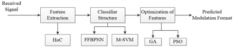
Figure 2(a) and 2(b) depicts the generalized system model for AMC. The signal is injected into the modulator for modulation subsequently, signal is transmitted over the channel. The additive white Guassain noise (AWGN) is considered throughout the research with different fading channel model i.e. Rayleigh and Rician. At the receiver side, features taken are higher order cumulants (HOC) extracted from the noisy received signal (Figure 3). Once features extracted, then these features are fed into the classifier [36]. The classifier structure is based on support vector machine (SVM) and feed forward back propagation neural network (FFBPNN). After that, the classifier performance is optimized using one of the famous heuristic computational technique i.e. Genetic Algorithm (GA) and particle swarm optimization (PSO). The generalized expression for received signal is given as below:
$r_{n}=s_{n}+g_{n}$ (1)
where, rn is the received baseband signal, gn is the additive white Gaussian Noise, sn is the transmitted signal and is defined as
$s_{n}=\mathrm{K} e^{-i\left(2 \pi f_{0} n T+\theta_{0}\right)} \sum_{j=-\infty}^{j=\infty} S(l) h(n T-j T+\left.\in_{T} T\right)$ (2)
where, S(l) is sequence of symbols at the input that is taken out from the set of M constellations of known symbols and the condition for symbols to be equiprobable is not necessary, K is the signal amplitude, f0 is offset constant of frequency, T is the spacing of symbols, θn is phase jitter which differs from symbol to symbol, h is channel effects and $\in_{T}$ is jitter timing.
Figure 2. Transmitter side of proposed system model
Figure 3. Receiver side for proposed system model
Table 2. Theoretical values of higher order moments and cumulants
|
|
QAM2 |
QAM4 |
QAM8 |
QAM16 |
QAM32 |
QAM64 |
|
M20 |
1 |
0.1 |
3.8 |
0.36 |
0.9 |
0.73 |
|
M21 |
2 |
0.1 |
0.8 |
0.04 |
0.08 |
0.04 |
|
M40 |
2 |
0.9 |
0.9 |
0.73 |
0.2 |
0.62 |
|
M42 |
0 |
6.9 |
68.4 |
203 |
748.8 |
3535.26 |
|
M60 |
0.02 |
0.09 |
0.12 |
0.2 |
0.13 |
0.32 |
|
M63 |
1 |
2.8 |
16.8 |
36.3 |
96.1 |
312.5 |
|
M84 |
1 |
4 |
11.6 |
75.89 |
78.80 |
1108.5 |
|
C20 |
1 |
0.1 |
3.8 |
0.36 |
0.98 |
0.73 |
|
C21 |
1 |
2 |
5.8 |
10.1 |
19.3 |
42.04 |
|
C40 |
2 |
0.9 |
0.9 |
0.73 |
0.21 |
0.62 |
|
C42 |
2 |
1 |
0.9 |
0.66 |
0.67 |
0.61 |
The representation of pth order of Cumulants is same as pth order of moment.
$C_{p q}=\operatorname{cum}[\underbrace{s, \ldots \ldots, S}_{(p-q) \text { terms }}, \quad \underbrace{s^{*}, \ldots . s^{*}}_{(q) \text { terms }}]$ (3)
The nth order Cumulants is the function of the moments order up to n
$\operatorname{cumm}\left[s_{1}, \ldots . ., s_{n}\right]=\sum_{\forall v}(-1)^{q-1}(q-1) ! E\left[\prod_{j \in v 1} s_{j}\right] \ldots E\left[\prod_{j \in v_{q}} s_{j}\right]$ (4)
The features selected for classification of M-QAM signals are as under [37]:
$C_{20}=\mathrm{E}\left[y^{2}(n)\right]=\operatorname{cumm}\{\mathrm{y}(\mathrm{n}), \mathrm{y}(\mathrm{n})\}$ (5)
$C_{21}=\mathrm{E}\left[|y(n)|^{2}\right]=\operatorname{cumm}\left\{\mathrm{y}(\mathrm{n}), y^{*}(n)\right\}$ (6)
$C_{40}=M_{40}-3 M_{20}^{2}=\operatorname{cumm}\{\mathrm{y}(\mathrm{n}), \mathrm{y}(\mathrm{n}), \mathrm{y}(\mathrm{n}), \mathrm{y}(\mathrm{n})\}$ (7)
$C_{41}=M_{40}-3 M_{20} M_{21}=\operatorname{cumm}\left\{\mathrm{y}(\mathrm{n}), \mathrm{y}(\mathrm{n}), \mathrm{y}(\mathrm{n}), y^{*}(n)\right\}$ (8)
$\begin{aligned} C_{42}=M_{42}-\left|M_{20}\right|^{2} &-2 M_{21} = \operatorname{cumm}\left\{\mathrm{y}(\mathrm{n}), \mathrm{y}(\mathrm{n}), y^{*}(n), y^{*}(n)\right\} \end{aligned}$ (9)
$M_{p q}=\mathrm{E}\left[s^{p-q}\left(s^{*}\right)^{q}\right]$ (10)
whereas, p represents the order of moment and s∗ is the complex conjugate of a signal s. C2,0 is the second order cumulants, which is known as the expected value of the square of the received signal also known as the mean. C2,1 is the class of second order cumulants, which represents the expected value of the absolute square of the received signal. C4,0 is the forth order cumulants, with no absolute value of the received signal basically, it is the combination of the M4,0 and M4,1. Similarly C4,1 and C4,2 is the class of 4th order cumulants. The theoretical values of the Cumulants are shown in Table 2.
After the features extraction from the noisy signal, these features are now input to the classifier structure. The classifier is based on multi-class SVM. SVM has a solid mathematical model, which can efficiently resolve the construction problem of high dimensional data model in the finite set of samples, and can converge to global best [38].
The SVM basics for solving the best linear hyper plane which could classify all the signals completely. Considered the training data as below:
$\left.\left\{\left(x_{1}, y_{1}\right), x_{2}, y_{2}\right), \ldots\left(x_{i}, y_{i}\right), x \in \operatorname{Rd}, y \in\{+1,-1\}\right\}$ (11)
whereas, xi represent the feature space, yi= +1 means that the signal belongs to the first class, yi= −1 shows that the signal is member of second class. Such kind of data are separated through hyper plane w*x+b = 0, when training data is linearly distinguishable. Then the solution for optimal plane problem is the optimization problem.
Minimize ½ ||$w \|^{2}$, with reference to yi (w.xi + b) ≥ 1, Lagrange multiplier is introduced for solving the quadratic programming problems and the best decision function is obtained by,
$f_{x}=\operatorname{sign}\left[\sum_{i=1}^{n} \alpha_{i} y_{i}\left(x_{i}, x\right)+b\right]$ (12)
whereas, αi is known as Lagrange multiplier. For classification of nonlinear data, SVM make comparison by nonlinearly of training data with high dimensional feature space through its kernel function afterwards it is processed as linear classification. Decision function is given as [39]:
$f_{x}=\operatorname{sign}\left[\sum_{i=1}^{n} \alpha_{i} y_{i} k\left(x_{i}, x\right)+b\right]$ (13)
whereas, k(xi, x)indicates kernel function. The typical kernel functions consist of the radial basis function (RBF):
$\mathrm{K}(\mathrm{x}, \mathrm{y})=\exp \left(-\|\mathrm{x}-\mathrm{y}\|^{2} / 2 \sigma^{2}\right)$ (14)
In short, Modulation classification based on SVM includes the followings steps:
To optimize the classification accuracy of SVM based classifier, Genetic Algorithm is used in conjunction with SVM. In this research, the extracted features are optimized in such a way to minimize the mean square error between the theoretical values and original values of the features. The cost function for the GA is mean square error and can be expressed as follows:
$J=\frac{1}{N} \sum_{k=1}^{N} e_{k}(n)^{2}$ (15)
where, J corresponds the mean square error (MSE). The fitness function (FF) for the GA is defined as [40]:
$F F=\frac{1}{1+J} ; \quad 0<F<1$ (16)
The genetic algorithm is used to minimize the cost as discussed in Eq. (15) or maximize the fitness function as shown in Eq. (16). The algorithm to optimize the features for SVM are shown in the following steps: -
Step-1: Initialize random population (selected features)
Step-2: Calculate fitness function of each candidate solution (using Eq. (16))
Step-3: Select best-ranking candidates to mate pairs at random
Step-4: Apply single point crossover operator
Step-5: Calculate fitness function of each new population (using Eq. (16)) & Apply mutation operator (optional)
Step-6: Check whether the terminating condition fulfilled (e.g. desired fitness achieved or enough number of cycles completed), If yes then terminate algorithm otherwise go to step 3.
The pseudo code of proposed optimized features for SVM are shown in Table 3.
Table 3. Pseudo code of proposed algorithm
|
while do if initialization ~ done continue //Parameter Initialization else break // Move to next step end |
|
for i = 1:N for j=1:M // N is the length of HOC (Rows) // M => # of columns end If Higher_Order_Cummulants ==true break else continue initialization end end // Generate signal and extract features |
|
while Iterations_left do for k = 1:length(Iterations) if algorithm_type==GA Apply GA // Steps are given in section 3 end save fitness end if MSE == MSE_desired break else continue // Keep running the algorithm until desired MSE is found |
|
Apply SVM for Classification End // Save all the results in tabular/graphical form |
In this paper, different QAM’s modulation schemes are simulated in the MATLAB. Different noises i.e. AWGN noise, Rician flat fading and Rayleigh flat fading noises are added in the transmitted signals data. The simulation is performed with different number of samples (NoS) on each channel at SNR’s. The simulation shows the average classification accuracy of QAM modulation format. For classification purpose, support vector machine (SVM) classifier is used. For this, 50% of samples are used for testing, 30% samples are used for testing and 20% samples are used for validation purpose. The figure of merit for the problem is average classification accuracy (ACA). The simulation parameters are shown in Table 4.
Table 4. Simulation parameters for optimization of features
|
Genetic Algorithm Parameters |
Values |
|
Candidate Solutions |
10-50 |
|
Cross-over |
Single Point |
|
Fitness Scaling |
Rank |
|
Selection |
Roulette Wheel |
|
Mutation |
Adaptive Feasible |
|
Hybrid Function |
NA |
|
Stoppage Criterion |
FF=0.99 |
|
Iterations |
1000 |
|
SNR in dB |
0-5 dB |
4.1 ACA without optimization
Table 4 shows the training and testing of average classification accuracy on different channels with different number of samples at different SNR values. Table 5 also shows that the classification accuracy increases as the number of samples are increased and it also increases by increasing the SNR. Moreover, it is also clear from Table 5 that AWGN channel has better classification accuracy than the Rician flat fading channel and Rayleigh flat fading channels, because AWGN noise is linear to the communication channel. Moreover, Rayleigh channel has less classification accuracy than AWGN and Rician, it is due to unavailability of line of sight (LOS) path between sender and receiver. The percentage classification accuracy reaches from 91.98% to 97.54%, when 4096 number of samples are taken in AWGN channel model. Also, it is reaches to 95.75% and 94.50% for Rician and Rayleigh channels respectively, having same number of samples and at 5 dB SNR.
4.2 ACA with optimization
Table 6 shows the percentage classification accuracy of training and testing of classifier at different SNR‘s, with different number of samples, by applying Genetic Algorithm. For 512 number of samples classification accuracy become 92.1% at 0 dB SNR for AWGN channel. Also, for 5 dB it reaches to 94.5% for same number of samples and same channel model. Moreover, for 4096 samples it approaches to 97.2% for 0 dB SNR and 98.6% at 5 dB SNR. However, for Rician channel it reaches to 96.7% on 512 samples at 10dB SNR and 98.6% when 4096 samples are taken, for same value of SNR. Also, for Rayleigh channel, percentage classification accuracy also increased and it reaches to 98.7% at 5 dB SNR, when 4096 samples are taken.
Table 5. ACA without optimization
|
Channel |
No. of Samples |
Training |
Testing |
||
|
0 dB |
5 dB |
0 dB |
5dB |
||
|
AWGN |
512 |
94.15 |
95.20 |
90.83 |
91.98 |
|
1024 |
95.34 |
96.85 |
92.74 |
93.86 |
|
|
2048 |
96.81 |
97.6 |
96.14 |
96.52 |
|
|
4096 |
97.26 |
98.75 |
97.00 |
97.54 |
|
|
Rician |
512 |
93.93 |
94.13 |
90.24 |
91.65 |
|
1024 |
94.85 |
95.7 |
91.7 |
93.21 |
|
|
2048 |
95.73 |
95.95 |
93.15 |
93.74 |
|
|
4096 |
96.83 |
96.75 |
94.24 |
95.75 |
|
|
Rayleigh |
512 |
92.83 |
94.11 |
87.9 |
91.25 |
|
1024 |
93.05 |
94.98 |
87.95 |
92.89 |
|
|
2048 |
93.86 |
95.46 |
91.25 |
93.52 |
|
|
4096 |
94.54 |
96.24 |
92.42 |
94.50 |
|
|
Channel |
No. of Samples |
Training |
Testing |
||
|
WOO |
WO |
WOO |
WO |
||
|
AWGN |
512 |
94.15 |
96.3 |
90.83 |
92.1 |
|
1024 |
95.34 |
97.4 |
92.74 |
95.6 |
|
|
2048 |
96.81 |
97.9 |
96.14 |
98.1 |
|
|
4096 |
97.26 |
99.5 |
97 |
99.2 |
|
|
Rician |
512 |
93.93 |
95.1 |
90.24 |
93.2 |
|
1024 |
94.85 |
96.8 |
91.7 |
96.5 |
|
|
2048 |
95.73 |
97.9 |
93.15 |
97.0 |
|
|
4096 |
96.83 |
98.1 |
94.24 |
97.2 |
|
|
Rayleigh |
512 |
92.83 |
95.1 |
87.9 |
92.1 |
|
1024 |
93.05 |
96.7 |
87.95 |
93.4 |
|
|
2048 |
93.86 |
97.3 |
91.25 |
94.2 |
|
|
4096 |
94.54 |
97.9 |
92.42 |
95.3 |
|
Table 7 shows the comparison of classification accuracy of both training and testing for each channel model at 0 dB SNR. On AWGN channel model, the classification accuracy without optimization (WOO) of training and testing was 94.15% and 90.83% respectively, when 512 samples are used for simulation. After applying GA, this classification rate is improved and training and testing reaches to 96.3% and 92.1% respectively. And for 1024, 95.34 to 97.4% for testing and for training 92.74% to 93.6%. The accuracy rate for 2048 number of samples is 96.81% to 97.9% for training and for testing it reaches from 96.14 % to 98.1 %. When 4096 samples are used, we achieve highest accuracy rate, at this SNR. The table shows that training accuracy of training approaches to 97.26% to 99.5% and for testing approaches to 97% to 99.2%. Although, Rician channel has not good accuracy as compared to AWGN channel model accuracy but it also increases the classification accuracy after optimization by using GA. For training, classification accuracy with 512, 1024, 2048 and 4096 samples turn into 95.1, 96.8, 97.9 and 98.1% respectively. And for testing, it reaches to 93.2, 96.5, 97 and 97.2% for respective number of samples. Also, the classification accuracy increases with optimization (WO) in the Rayleigh channel model for both training and testing. When 512 samples are taken, classification accuracy of training reaches to 95.1% and for testing it reaches to 92.1% and for 4096 number of samples, it increases to 97.9% and 95.3% for training and testing respectively.
Table 7. Average classification accuracy at 0 dB
|
Channel |
No. of Samples |
Training |
Testing |
||
|
0 dB |
5 dB |
0 dB |
5 dB |
||
|
AWGN |
512 |
96.3 |
97.4 |
92.1 |
94.5 |
|
1024 |
97.4 |
99.1 |
93.6 |
97.7 |
|
|
2048 |
97.9 |
99.3 |
98.1 |
98.6 |
|
|
4096 |
99.5 |
99.9 |
99.2 |
99.9 |
|
|
Rician |
512 |
95.1 |
96.5 |
93.2 |
96.7 |
|
1024 |
96.8 |
97.2 |
96.5 |
97.8 |
|
|
2048 |
97.9 |
98.3 |
97.0 |
98.1 |
|
|
4096 |
98.1 |
98.7 |
97.2 |
98.6 |
|
|
Rayleigh |
512 |
95.1 |
96.5 |
92.1 |
93.5 |
|
1024 |
96.7 |
97.8 |
93.4 |
96.3 |
|
|
2048 |
97.3 |
98.4 |
94.15 |
97.9 |
|
|
4096 |
97.9 |
98.5 |
95.3 |
98.2 |
|
Table 8 shows the comparison of classification accuracy on different channel models with different number of samples at 5 dB SNR. The table shows that classification accuracy rises after optimization. It shows that the percentage classification accuracy also reaches to 99.9% both for training and testing after applying Genetic Algorithm, when 4096 samples are used. The classification accuracy for Rician channel reaches to 98.7% and 98.6% for training and testing respectively, on same number of samples. However, the classification accuracy on Rayleigh channel also increases and reaches to 98.5% and 98.2%. When we compare the result of Table 7 with Table 6 results, it is also clear that the Table 7 has better classification accuracy rate than the classification accuracy result in Table 6, for all channel model as well as for each number of samples on every channel model.
Table 8. Average classification accuracy at 5 dB
|
Channel |
No. of Samples |
Training |
Testing |
||
|
WOO |
WO |
WOO |
WO |
||
|
AWGN |
512 |
95.2 |
97.4 |
91.98 |
94.5 |
|
1024 |
96.85 |
99.1 |
96.68 |
98.7 |
|
|
2048 |
97.6 |
99.3 |
96.52 |
98.6 |
|
|
4096 |
98.75 |
99.9 |
97.54 |
99.9 |
|
|
Rician |
512 |
94.13 |
96.5 |
91.65 |
96.7 |
|
1024 |
95.7 |
97.2 |
93.21 |
97.8 |
|
|
2048 |
95.95 |
98.3 |
93.74 |
98.1 |
|
|
4096 |
96.75 |
98.7 |
95.75 |
98.6 |
|
|
Rayleigh |
512 |
94.11 |
96.5 |
91.25 |
93.5 |
|
1024 |
94.98 |
97.8 |
92.89 |
96.3 |
|
|
2048 |
95.46 |
98.4 |
93.52 |
97.9 |
|
|
4096 |
96.24 |
98.5 |
94.50 |
98.2 |
|
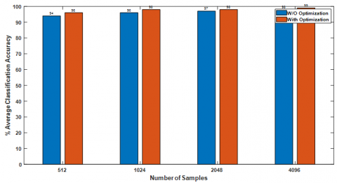
The performance comparison with and without optimization on AWGN channel, Rician channel and Rayleigh channel are shown in Figures 4-6 respectively. The Figures 4-6, shows the average classification accuracy (ACA) on different number of samples i.e. 512, 1024, 2048 & 4096. As it clear from the Figures 4-6, the average classification accuracy with optimization is quite better than the without optimization.
Figure 4. Percentage ACA on AWGN channel
Figure 5. Percentage ACA on rician channel
Figure 6. Percentage ACA on Rayleigh channel
4.5 ACA comparison with existing techniques
Table 9 shows the training and testing accuracy of proposed and existing classifier, and it is found that proposed classifier performs better in both scenarios also at lower SNR’s. The performance of the proposed GA-SVM classifier is compared with the state of art existing technique [33]. Table 9 shows the training and testing accuracy of proposed and existing classifier, and it is found that proposed classifier performs better in both scenarios also at lower SNR’s. At 5 dB of SNR, the proposed classifier gives percentage ACA of 99.12 and 98.71 for training and testing respectively, while when compared the existing algorithm have percentage ACA of 98.95 and 98.75 respectively.
In Table 10, the comparison of percentage ACA with the existing techniques at 0 dB and 5 dB of SNR with 4096 number of samples on AWGN channel with optimization. The performance is compared and found the proposed classifier performance is better and approximately approaching to 100% at lower SNR’s. Table 11, shows the performance comparison of proposed classifier structure with the state of art existing techniques. The proposed classifier performs much better as compared to the existing techniques.
Table 9. ACA comparison with [33]
|
Channel/No of Samples |
0 dB without Optimization |
|||
|
Training [33] |
Training [Proposed] |
Testing [33] |
Testing [Proposed] |
|
|
AWGN
1024 |
93.26 |
95.34 |
91.45 |
92.74 |
|
5 dB without Optimization |
||||
|
96.75 |
96.85 |
96.54 |
96.68 |
|
|
0 dB with Optimization |
||||
|
94.92 |
97.40 |
93.64 |
95.6 |
|
|
5 dB with Optimization |
||||
|
98.95 |
99.12 |
98.75 |
98.71 |
|
Table 10. ACA comparison with [28, 39]
|
Channel/No of Samples |
0dB [39] |
0dB Proposed |
5dB [39] |
5dB Proposed |
|
AWGN 4096 |
98.48 |
99.21 |
99.86 |
99.93 |
|
0dB [28] |
0dB Proposed |
5dB [28] |
5dB Proposed |
|
|
96.30 |
99.21 |
98.95 |
99.93 |
Table 11. ACA comparison with the state of art existing techniques
|
Reference |
No. of samples |
SNR Value |
Previous ACA |
Proposed ACA |
|
[40] |
1024 |
0dB |
57.2% |
96.2% |
|
10dB |
75.36% |
99.1% |
||
|
[2] |
512 |
0dB |
92.7% |
94.12% |
|
[18] |
512 |
10dB |
88% |
97.4% |
|
[23] |
1024 |
0dB |
89.3% |
96.2% |
|
5dB |
96.1% |
97.4% |
||
|
[9] |
2048 |
10dB |
97.7% |
99.3% |
|
[16] |
512 |
0dB |
78.4% |
95.1% |
|
5dB |
93.3% |
96.4% |
||
|
10dB |
96.4% |
97.4% |
||
|
[37] |
512 |
0dB |
80.9% |
96.3% |
|
5dB |
96.4% |
97.4% |
||
|
[25] |
4096 |
0dB |
96.3% |
99.21% |
|
5dB |
98.95% |
99.93% |
||
|
[24] |
4096 |
0dB |
98.48% |
99.21% |
|
5dB |
99.86% |
99.93% |
AMC has vast significance in enhancing the consumption of the available band and enhancing the communication systems throughput. The likelihood based AMC is optimal but difficult to implement on the other hand features based pattern recognition approach is simple to implement. For AMC higher order cumulants based features are used and AMC is executed by combining SVM and GA. Simulation results is demonstrated under AWGN, Rayleigh and Rician noise of different values of SNR’s. It has been found that percentage accuracy of classification is higher at low SNR’s also percentage accuracy of optimized classifier increases significantly as compared than the simple classifier. In future different classifier structure such as radial basis function and committee machines with reduced feature set may be utilized for better classification accuracy.
[1] Zhao, J.L., Wang, T.T. (2011). Identification of cognitive radio modulation. In 2011 International Conference on Mechatronic Science, Electric Engineering and Computer (MEC), pp. 1773-1776. https://doi.org/10.1109/mec.2011.6025826
[2] Liu, J., Luo, Q. (2012). A novel modulation classification algorithm based on daubechies5 wavelet and fractional Fourier transform in cognitive radio. In 2012 IEEE 14th International Conference on Communication Technology, pp. 115-120. https://doi.org/10.1109/icct.2012.6511199
[3] Castro, A.R., Freitas, L.C., Cardoso, C.C., Costa, J.C., Klautau, A.B. (2012). Modulation classification in cognitive radio. Foundation of Cognitive Radio Systems, 43. https://doi.org/10.5772/30764
[4] Ghauri, S.A., Qureshi, I.M., Cheema, T.A., Malik, A.N. (2014). A novel modulation classification approach using Gabor filter network. The Scientific World Journal, 2014: 643671. https://doi.org/10.1155/2014/643671
[5] Ghauri, S.A., Mansoor Qureshi, I. (2015). PAM signals classification using modified Gabor filter network. Mathematical Problems in Engineering, 2015: 262180. https://doi.org/10.1155/2015/262180
[6] Ghauri, S.A., Qureshi, I.M., Shah, I., Khan, N. (2014). Modulation classification using cyclostationary features on fading channels. Research Journal of Applied Sciences, Engineering and Technology, 7(24): 5331-5339. https://doi.org/10.19026/rjaset.7.932
[7] Dobre, O.A., Abdi, A., Bar-Ness, Y., Su, W. (2007). Survey of automatic modulation classification techniques: Classical approaches and new trends. IET Communications, 1(2): 137-156. https://doi.org/10.1049/iet-com:20050176
[8] Morales-Jimenez, D., Gomez, G., Paris, J.F., Entrambasaguas, J.T. (2009). Joint adaptive modulation and MIMO transmission for Non-Ideal OFDMA cellular systems. 2009 IEEE Globecom Workshops, Honolulu, HI, USA, pp. 1-5. https://doi.org/10.1109/glocomw.2009.5360728
[9] Ye, Z., Memik, G., Grosspietsch, J. (2007). Digital modulation classification using temporal waveform features for cognitive radios. 2007 IEEE 18th International Symposium on Personal, Indoor and Mobile Radio Communications, pp. 1-5. https://doi.org/10.1109/pimrc. 2007.4394558
[10] Hameed, F., Dobre, O., Popescu, D. (2009). On the likelihood-based approach to modulation classification. IEEE Transactions on Wireless Communications, 8(12): 5884-5892. https://doi.org/10.1109/twc.2009.12.080883
[11] Xu, J.L., Su, W., Zhou, M. (2011). Likelihood-Ratio approaches to automatic modulation classification. IEEE Transactions on Systems, Man, and Cybernetics, Part C (Applications and Reviews), 41(4): 455-469. https://doi.org/10.1109/tsmcc.2010.2076347
[12] Bai, D., Lee, J., Kim, S., Kang, I. (2012). Near ML modulation classification. In 2012 IEEE Vehicular Technology Conference (VTC Fall), pp. 1-5. https://doi.org/10.1109/vtcfall.2012.6398878
[13] Shi, Q., Karasawa, Y. (2011). Noncoherent maximum likelihood classification of quadrature amplitude modulation constellations: Simplification, analysis, and extension. IEEE Transactions on Wireless Communications, 10(4): 1312-1322. https://doi.org/10.1109/twc. 2011.030311.101490
[14] Wang, F., Wang, X. (2010). Fast and robust modulation classification via Kolmogorov-Smirnov test. IEEE Transactions on Communications, 58(8): 2324-2332. https://doi.org/10.1109/tcomm.2010.08.090481
[15] Liu, A.S., Qi, Z.H.U. (2011). Automatic modulation classification based on the combination of clustering and neural network. The Journal of China Universities of Posts and Telecommunications, 18(4): 13-38. https://doi.org/10.1016/s1005-8885(10)60077-5
[16] Zhu, Z., Nandi, A.K. (2014). Blind digital modulation classification using minimum distance centroid estimator and Non-Parametric likelihood function. IEEE Transactions on Wireless Communications, 13(8): 4483-4494. https://doi.org/10.1109/twc.2014.2320724
[17] Le, B., Rondeau, T.W., Maldonado, D., Bostian, C.W. (2005). Modulation identification using neural network for cognitive radios. In Software Defined Radio Forum Technical Conference.
[18] Muhlhaus, M.S., Oner, M., Dobre, O.A., Jondral, F.K. (2013). A low complexity modulation classification algorithm for MIMO systems. IEEE Communications Letters, 17(10): 1881-1884. https://doi.org/10.1109/LCOMM.2013.091113.130975
[19] Ramezani-Kebrya, A., Kim, I.M., Kim, D.I., Chan, F., Inkol, R. (2013). Likelihood-Based modulation classification for multiple-antenna receiver. IEEE Transactions on Communications, 61(9): 3816-3829. https://doi.org/10.1109/tcomm.2013.073113.121001
[20] Huang, S., Yao, Y., Wei, Z., Feng, Z., Zhang, P. (2017). Automatic modulation classification of overlapped sources using multiple cumulants. IEEE Transactions on Vehicular Technology, 66(7): 6089-6101. https://doi.org/10.1109/tvt.2016.2636324
[21] Orlic, V., Dukic, M. (2009). Automatic modulation classification algorithm using higher-order cumulants under real-world channel conditions. IEEE Communications Letters, 13(12): 917-919. https://doi.org/10.1109/lcomm.2009.12.091711
[22] Gong, X., Li, B., Zhu, Q. (2010). Collaborative modulation recognition based on SVM. 2010 Sixth International Conference on Natural Computation, 2: 871-874. https://doi.org/10.1109/icnc.2010.5583916
[23] Sherme, A.E. (2012). A novel method for automatic modulation recognition. Applied Soft Computing, 12(1): 453-461. https://doi.org/10.1016/j.asoc.2011.08.025
[24] Ebrahimzadeh, A., Ghazalian, R. (2011). Blind digital modulation classification in software radio using the optimized classifier and feature subset selection. Engineering Applications of Artificial Intelligence, 24(1): 50-59. https://doi.org/10.1016/j.engappai.2010.08.008
[25] Su, W. (2013). Feature space analysis of modulation classification using very high-order statistics. IEEE Communications Letters, 17(9): 1688-1691. https://doi.org/ 10.1109/lcomm. 2013. 080613.130070
[26] Zaerin, M., Seyfe, B. (2012). Multiuser modulation classification based on cumulants in additive white Gaussian noise channel. IET Signal Processing, 6(9): 815-823. https://doi.org/10.1049/iet-spr.2011.0357
[27] Hussain, A., Sohail, M.F., Alam, S., Ghauri, S.A., Qureshi, I.M. (2019). Classification of M-QAM and M-PSK signals using genetic programming (GP). Neural Computing and Applications, 31(10): 6141-6149. https://doi.org/10.1007/s00521-018-3433-1
[28] Gupta, R., Kumar, S., Majhi, S. (2020). Blind modulation classification for asynchronous OFDM systems over unknown signal parameters and channel statistics. IEEE Transactions on Vehicular Technology, p. 1. https://doi.org/10.1109/tvt.2020.2981935
[29] Wang, Y., Gui, J., Yin, Y., Wang, J., Sun, J., Gui, G., Adachi, F. (2020). Automatic modulation classification for MIMO systems via deep learning and zero-forcing equalization. IEEE Transactions on Vehicular Technology, 69(5): 5688-5692. https://doi.org/10.1109/tvt.2020.2981995
[30] Zhu, Z., Waqar Aslam, M., Nandi, A.K. (2014). Genetic algorithm optimized distribution sampling test for M-QAM modulation classification. Signal Processing, 94: 264-277. https://doi.org/10.1016/j.sigpro.2013.05.024
[31] Maclellan, A., McLaughlin, L., Crockett, L., Stewart, R. (2019). FPGA accelerated deep learning radio modulation classification using MATLAB system objects PYNQ. 2019 29th International Conference on Field Programmable Logic and Applications (FPL), pp. 246-247 https://doi.org/10.1109/fpl.2019.00045
[32] Huang, S., Jiang, Y., Gao, Y., Feng, Z., Zhang, P. (2019). Automatic modulation classification using contrastive fully convolutional network. IEEE Wireless Communications Letters, 8(4): 1044-1047. https://doi.org/10.1109/lwc.2019.2904956
[33] Abdelmutalab, A., Assaleh, K., El-Tarhuni, M. (2016). Automatic modulation classification based on high order cumulants and hierarchical polynomial classifiers. Physical Communication, 21: 10-18. https://doi.org/10.1016/j.phycom.2016.08.001
[34] Tu, Y., Lin, Y., Hou, C., Mao, S. (2020). Complex-valued networks for automatic modulation classification. IEEE Transactions on Vehicular Technology, p. 1. https://doi.org/10.1109/TVT.2020.3005707
[35] Wang, Y., Gui, G., Gacanin, H., Ohtsuki, T., Sari, H., Adachi, F. (2020). Transfer learning for semi-supervised automatic modulation classification in ZF-MIMO systems. IEEE Journal on Emerging and Selected Topics in Circuits and Systems, p. 1. https://doi.org/10.1109/jetcas. 2020.2992128
[36] El-Khoribi, R.A., Shoman, M.A.I., Mohammed, A.G.A. (2014). Automatic digital modulation recognition using artificial neural network in cognitive radio. International Journal of Emerging Trends & Technology in Computer Science, 3(3): 132-136.
[37] Hussain, A., Ghauri, S.A., Qureshi, I.M., Sohail, M.F., Khan, S.A. (2016). KNN based classification of digital modulated signals. IIUM Engineering Journal, 17(2): 71-82. https://doi.org/10.31436/iiumej.v17i2.641
[38] Peng, S., Jiang, H., Wang, H., Alwageed, H., Zhou, Y., Sebdani, M.M., Yao, Y.D. (2018). Modulation classification based on signal constellation diagrams and deep learning. IEEE Transactions on Neural Networks and Learning Systems, 30(3): 718-727. https://doi.org/10.1109 /tnnls.2018.2850703
[39] Ghauri, S.A., Shah, H.H., Sajjad, H. (2013). Comparison of different population strategies for multiuser detection using Genetic Algorithm. World Congress on Internet Security (WorldCIS-2013), pp. 65-68. https://doi.org/10.1109/worldcis.2013.6751018
[40] Ozen, A., Ozturk, C. (2013). A novel modulation recognition technique based on artificial bee colony algorithm in the presence of multipath fading channels. 2013 36th International Conference on Telecommunications and Signal Processing (TSP), pp. 239-243. https://doi.org/10.1109/tsp.2013.6613928