Hussain Ali Azzawi* | Sabah A. Gitaffa![]() | Nihad M. Ameen
| Nihad M. Ameen
© 2023 IIETA. This article is published by IIETA and is licensed under the CC BY 4.0 license (http://creativecommons.org/licenses/by/4.0/).
OPEN ACCESS
As the impacts of global warming intensify, the automotive industry is increasingly emphasizing the development of eco-friendly vehicles with superior range and performance compared to conventional ones. Electric vehicles have emerged as a promising solution to reduce harmful emissions in the transportation sector. This study focuses on creating a nonlinear dynamic model for electric vehicles by integrating kinetic and electrical components. The key criterion in EV speed control is robustness, prompting the construction of various controllers to ensure resilience and disturbance rejection. These controllers include both traditional ones like proportional-integral-derivative (PID) and fractional order PID (FOPID) controllers. Fractional calculus has gained significant attention in control systems engineering due to the fractional orders of the integral and derivative terms, offering enhanced robustness and optimal control. This thesis employs multiple optimization strategies to design an FOPID controller, ensuring the optimal performance of a robust control system for electric vehicles. Initially, the controller is developed using intelligent swarm optimization techniques, such as particle swarm optimization (PSO) and grey wolf optimization (GWO), through simulations in MATLAB R2022b. The results demonstrate the effectiveness of PSO and GWO algorithms in reducing the objective integral of time multiplied by absolute error (ITAE) function in the speed control system utilizing an FOPID controller. The performance of a conventional PID controller is compared with that of a FOPID controller, highlighting the superiority of the GWO-FOPID strategy, presented as a novel methodology. The outcomes underscore the remarkable performance of the GWO-FOPID controller, ensuring rapid responsiveness in controlling EV speed, with a rise time of 0.008978 seconds, a settling time of 0.01 seconds, and zero absolute time error (ITAE).
fractional-order proportional-integral-derivative (FOPID), proportional-integral-derivative (PID), grey wolf optimization (GWO), particle swarm optimization (PSO), electric vehicles (EV), permanent magnet synchronous motors (PMSMs)
Due to environmental and energy concerns, electric vehicles are becoming an attractive alternative to traditional Vehicles with internal combustion engines. The research community has paid much attention to improving the performance of electric vehicles (EVs), which has also made progress in their design [1, 2]. A permanent magnet synchronous motor (PMSM) has been used in the design of electric vehicles as it has high energy density and efficiency. Therefore, it is suitable for high-performance applications [3]; PMSM are preferred by researchers and manufacturers over DC motors because of their many disadvantages. Thus, there is much room for improvement and development of a more compact intelligent swarm speed controller for PMSM drives [4, 5]. The controllers for electric vehicles have been the subject of numerous published studies. A gain-scheduled controller for the independent driving of four-wheel electric vehicle lateral stability was proposed by Xian J. Jin and coworkers in 2015 [6]. Khooban et al. [7] suggest an optimal multi-objective fuzzy fractional-order PIλ Dμ controller (MOFFOPID) for time-delayed EV. speed control. Simulation findings show the suggested controller performs well. Munoz-Hernandez et al. [8] present an electric vehicle cruise control design based on a fractional-order proportional and integral (PI) direct control of the torque applied to the propulsion system. Results from the simulation demonstrate the efficiency of the control. George et al. [9] propose an efficient adaptive neuro-fuzzy inference system (ANFIS)-based fractional order PID (FOPID) controller for an electric vehicle speed tracking control propelled by a DC motor. The proposed controller resists external disturbances and encourages speed regulation control for electric vehicles. The outcomes demonstrate the superior performance of the ANFIS-based FOPID controller with its high prediction and low error rates. Babaei et al. [10] introduced a negative swarm method (SSA) to modify the PID control coefficients (FOPID). Additionally, assessments of the suggested findings show that the FOPID controller may Greatly decrease overrun time and stability in Frequency change signals. This paper proposes to design a micro-arranged PID controller for an electric vehicle using PSO and GWO algorithms. The proposed design aims to improve the overall performance and efficiency of the electric vehicle control system. PSO and GWO algorithms optimize the controller parameters, resulting in an optimized control design. The effectiveness of the proposed controller design is evaluated through simulation studies. The results show that the design of the gray wolf controller is superior to the PSO, which indicates the effectiveness of the GWO algorithms in optimizing the partial arrangement of PID controllers for EVs.
The format of this essay is as follows: 2. Fractional order controller (FOC) and Mathematical Modeling of the EVs is the subject of Section 3. A summary of optimization methods and various metaheuristic PSO and GWO algorithms are provided in Section 4. Results from the tests are applied in Section 5. then highlights the conclusions of the proposed system.
A fractional differential equation or integral equation defines a fractional-order system, a concept beyond the scope of conventional calculus that focuses on integer-order differentiation and integration. Unlike traditional methods, fractional calculus allows differentiation and integration of any order, be it non-integer or integer. This approach has gained widespread acceptance across fields like fluid mechanics and electrical systems, becoming a significant method in engineering and science [11].
The incorporation of fractional order calculus into traditional controllers, like PI and PID, has significantly expanded performance capabilities. While traditional methods have dominated industrial applications, fractional order controllers have gained traction due to their precise modeling abilities. Initially, fractional order systems were approximated using integer models, but advancements in numerical methods have facilitated accurate representations using non-integer derivatives and integrals [12].
FOPID controllers, a notable application, have found use in electric vehicles, robotic systems, engines, and power systems. Despite their effectiveness, tuning FOPID controllers is challenging due to the additional parameters they introduce compared to traditional PID controllers. However, these parameters enhance the controller’s flexibility and design possibilities.
In the time domain, the FOPID controller is represented by the equation [13]:
$U(t)=K_p e(t)+K_i D^{-\lambda} e(t)+K_d D^\mu e(t)$ (1)
The Laplace transform provides a transfer function representation of FOPID as [9]:
$G_c(s)=\frac{u(s)}{e(s)}=K_p+K_i\left(s^{-\lambda}\right)+K_d\left(s^\mu\right)$ (2)
Figure 1. FOPID controller block diagram
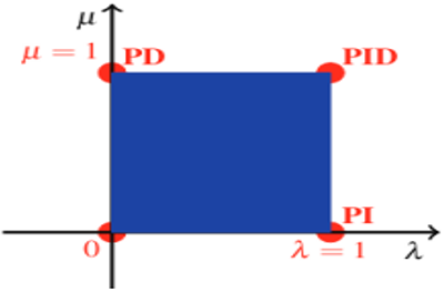
Figure 2. Operation region of the FOPID controller
The FOPID controller operates based on fractional power integral and differential terms represented by $\lambda$ and $\mu$, respectively as shown in the Figure 1. Various combinations of $\lambda$ and $\mu$ values can emulate classical controllers: $\lambda$ = 1, $\mu$ = 1 corresponds to the classical PID controller, $\lambda$ = 1, $\mu$ = 0 corresponds to the PI controller, and $\lambda$ = 0, $\mu$ = 1 corresponds to the PD controller. This relationship is visually represented in a two-dimensional plan, as depicted in Figure 2. The shaded area in blue indicates the fractional controller.
$G_c(s)=\frac{u(s)}{e(s)}=K_p+K_i\left(s^{-\lambda}\right)+K_d\left(s^\mu\right)$
where,
Gc(s): FOPID transfer function.
u(s): Controller output.
e(s): An error has been produced.
Kp, Ki, and Kd: the earnings equitably distributed, integral and derivative terms, respectively.
µ: Fractional portion of the derivative part.
λ: fractional component of the integral term.
3.1 Mechanical model
The EV consists primarily of a battery pack, a controller, and electric motors connected to the gearbox device. Vehicle and motor dynamics make up the EV system dynamics. Modelling the electric vehicle system involves balancing all forces acting on a moving vehicle. There are primarily four forms of forces: aerodynamic drag force (Fad), rolling friction (Frr), acceleration force (Fa) and gravitational force (Fg) [14] as depicted in Figure 3.
Figure 3. External forces are acting in EV
Aerodynamic force is:
$\mathrm{F}_{\text {area }}=\frac{1}{2} \rho \mathrm{AC}_{\mathrm{d}} \mathrm{v}^2$ (3)
Rolling force is:
$\mathrm{F}_{\text {tire }}=\mu_{\mathrm{rr}} \mathrm{mg}$ (4)
Hill climbing force is:
$\mathrm{F}_{\text {slope }}=\operatorname{mgsin}(\varphi)$ (5)
Acceleration force is:
$\mathrm{F}_{\text {acce }}=\mathrm{m} \frac{\mathrm{dv}}{\mathrm{dt}}$ (6)
Finally, the total force affected by the electric vehicle is:
$\mathrm{F}_{\mathrm{T}}=\mathrm{F}_{\text {area }}+\mathrm{F}_{\text {tire }}+\mathrm{F}_{\text {slope }}+\mathrm{F}_{\text {acce }}$ (7)
$\mathrm{F}_{\mathrm{T}}=\frac{1}{2} \rho \mathrm{AC}_{\mathrm{d}} \mathrm{v}^2+\mu_{\mathrm{rr}} \mathrm{mg}+\operatorname{mgsin}(\varphi)+\mathrm{m} \frac{\mathrm{dv}}{\mathrm{dt}}$ (8)
The velocity of the EV is denoted by v, the head portion of the car or truck is represented by A, the electric vehicle mass is m, the rolling resistance coefficient is μrr, g is the acceleration gravity, the density of the air is $\rho, \varphi$ is the angle at which the machine climbs a slope, and Cd is the coefficient of the drag operation [15].
The consequent force (FT) will result in a torque counterproductive to the driving motor, as illustrated by the following formula:
$\mathrm{T}_{\mathrm{L}}=\mathrm{F}_{\mathrm{T}}\left(\frac{\mathrm{r}}{\mathrm{G}}\right)$ (9)
where, G and r are the gearing ratio and tire radius of the EV, respectively, and the driving motor-produced torque is shown by TL [16].
3.2 Modeling of PMSM motor
The PMSM’s mathematical model can be expressed in a d-q reference frame rotating synchronously. This model is comparable to that of the wound rotor synchronous motor because the stator structures of both motors are similar. The PMSM’s model was created based on certain assumptions, including the neglect of saturation and the assumption that the induced EMF is sinusoidal. Eddy current and hysteresis losses are also considered negligible, and there are no current field dynamics. The resulting equations for the stator d and q components of the PMSM in the rotor reference frame can be derived from these assumptions [17].
$\mathrm{V}_{\mathrm{d}}=\mathrm{R}_{\mathrm{S}} \mathrm{i}_{\mathrm{d}}+\mathrm{p} \lambda_{\mathrm{d}}-\mathrm{w}_{\mathrm{e}} \lambda_{\mathrm{q}}$ (10)
$\mathrm{V}_{\mathrm{q}}=\mathrm{Rsi}_{\mathrm{q}}+\mathrm{p} \lambda_{\mathrm{q}}+\mathrm{w}_{\mathrm{e}} \lambda_{\mathrm{d}}$ (11)
$\mathrm{T}_{\mathrm{e}}=\left(\frac{3}{2}\right) \mathrm{P}\left(\lambda_{\mathrm{af}} \mathrm{i}_{\mathrm{q}}+\left(\mathrm{L}_{\mathrm{d}}-\mathrm{L}_{\mathrm{q}}\right) \mathrm{i}_{\mathrm{d}} \mathrm{i}_{\mathrm{q}}\right)$ (12)
$\mathrm{T}_{\mathrm{e}}=\mathrm{T}_{\mathrm{L}}+\mathrm{B} \mathrm{w}_{\mathrm{r}}+\mathrm{Jp} \mathrm{w}_{\mathrm{r}}$ (13)
$\mathrm{w}_{\mathrm{e}}=\mathrm{Pw}_{\mathrm{r}}$ (14)
where,
$\lambda_{\mathrm{q}}=\mathrm{L}_{\mathrm{q}} \mathrm{i}_{\mathrm{q}}$ (15)
$\lambda_{\mathrm{d}}=\mathrm{L}_{\mathrm{d}} \mathrm{i}_{\mathrm{q}}+\lambda_{\mathrm{af}}$ (16)
Voltages are represented by Vd and Vq, and currents by id and iq along the d and q axes, respectively. P stands for the number of pole pairs; Lq and Ld designate the inductances on the q and d axes, respectively; p is the derivative operator; TL and Te stands for the load and electric torques, and B stands for the damping coefficient. The mutual flux, also known as the airgap flux, is denoted by λaf, and J describes the inertial moment.
Assume all Eqs. (11) to (12) are nonlinear and that the vector-controlled PMSM forces the id variable to zero. Solving Eqs. (11) to (12) is shown below [18]:
$\mathrm{V}_{\mathrm{q}}=\mathrm{R}_{\mathrm{S}} \mathrm{i}_{\mathrm{q}}+\mathrm{L}_{\mathrm{q}} \mathrm{i}_{\mathrm{q}} \mathrm{P}+\mathrm{w}_{\mathrm{e}} \lambda_{\mathrm{af}}$ (17)
$\mathrm{V}_{\mathrm{d}}=-\mathrm{w}_{\mathrm{e}} \mathrm{L}_{\mathrm{q}} \mathrm{i}_{\mathrm{q}}$ (18)
$\mathrm{T}_{\mathrm{e}}=\left(\frac{3}{2}\right) \mathrm{P} \lambda_{\mathrm{af}} \mathrm{i}_{\mathrm{q}}-\mathrm{K}_{\mathrm{t}} \mathrm{i}_{\mathrm{q}}$ (19)
Transfer function of PMSM:
$\frac{\mathrm{w}_{\mathrm{r}}(\mathrm{S})}{\mathrm{V}_{\mathrm{q}}(\mathrm{S})}=\frac{\mathrm{K}_{\mathrm{t}}}{\left(\mathrm{R}+\mathrm{L}_{\mathrm{q}} \mathrm{S}\right)(\mathrm{JS}+\mathrm{B})+\mathrm{K}_{\mathrm{t}} \mathrm{P} \lambda_{\mathrm{af}}}$ (20)
Table 1. PMSM motor parameters [18]
|
Parameter |
Values |
Units |
|
Kt λaf Js R Lq B P |
6.807 1.513 0.0337 0.12 0.764 0.086 2 |
N-m/A V/rad/sec Kg-m2 Ω mH
pole pairs |
Table 1 shows the parameter values of the PMSM motor. These values are used in Eq. (20), we obtain Eq. (21).
$\frac{\mathrm{Wr}(\mathrm{S})}{\mathrm{V}_{\mathrm{q}}(\mathrm{S})}=\frac{6.807}{0.02257 \mathrm{s}^2+3.96 \mathrm{s}+20.6}$ (21)
Figure 4. Schematic of a permanent magnet synchronous motor
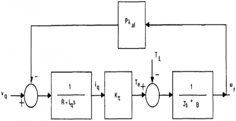
As depicted in Figure 4, the visual representation illustrates the connection of the Torque load to the synchronous motor, denoted as TL. Here, the Torque load signifies the combined torques influencing the electric vehicle's motion. Eq. (22) provides a detailed explanation of this scenario.
$\mathrm{T}_{\mathrm{L}}=\left(\frac{\mathrm{r}}{\mathrm{G}}\right)\left(\frac{1}{2} \rho \mathrm{AC}_{\mathrm{d}} \mathrm{v}^2+{\mathrm{\mu}}_{\mathrm{rr}} \mathrm{mg}+\mathrm{mgsin}(\varphi)+ \mathrm{m} \frac{\mathrm{dv}}{\mathrm{dt}}\right)$ (22)
It is recommended that appropriate nonlinear control strategies be utilized in developing the control system for these types of structures. Some process parameters are subject to change due to the broad range of process parameters, making accurate design an arduous task. As an illustration, the armature resistance of the motor is susceptible to change whenever there is a shift in the operating temperature. This underlines the importance of a resilient personality for the controller. Table 2 explains this research’s EV parameters and coefficients [18, 19].
Table 2. EV system’s parameters
|
Values |
Parameters |
Values |
Parameters |
Values |
Parameters |
Values |
Parameters |
|
0.764 |
Lq (mH) |
35◦ |
φ (◦) |
0.015 |
μrr |
2800 |
ωnom |
|
0.086 |
B |
6.807 |
Kt (N-m/A) |
11 |
G |
800 |
m (kg) |
|
2 |
P |
1.513 |
λaf (V/rad/sec) |
0.0002 |
B (N.M.s) |
1.8 |
A (m2) |
|
|
|
0.0337 |
Js (Kg-m2) |
78 |
I (A) |
1.25 |
ρ (kg/m2) |
|
|
|
0.12 |
R (Ω) |
0~48 |
V (volt) |
0.3 |
Cd |
Intelligent swarms, refer to systems composed of multiple autonomous agents that can interact and collaborate with each other to accomplish complex tasks. These swarms are often inspired by the collective behavior observed in natural systems such as ant colonies, bird flocks, and bee hives. Intelligent swarms typically consist of a large number of simple individual agents that follow local rules and communicate with their neighbors. Through these local interactions and communication, they exhibit emergent behavior, which leads to complex and intelligent global behavior of the entire swarm, make decisions based on local information, and coordinate their actions with other agents to achieve specific goals [20]. These swarms can be applied in various domains, including robotics, artificial intelligence, optimization, and logistics. Intelligent swarms have the advantage of being robust, scalable, and adaptable. Even if individual agents fail or are removed from the swarm, the overall system can continue to function. Additionally, these swarms can exhibit emergent properties and self-organization, allowing them to adapt to changing environments and tasks [21].
However, there are also challenges associated with intelligent swarms, including coordination, communication, scalability, and ensuring the swarm’s behavior aligns with desired objectives. Research in this field continues to advance our understanding of swarm intelligence and develop practical applications for these systems.
4.1 Grey wolf optimization (GWO)
In 2014, Mirjalili et al. [22] developed the Grey Wolf Optimizer (GWO) by modelling the hierarchy and hunting organization of the Grey Wolf. Aims to enhance efficiency in controller design, addressing the need for a more optimized approach, leveraging the insights from grey wolf behavior for optimization strategies. The strategy utilized exemplifies grey wolf communities’ hierarchical social structure and cooperative hunting behavior [22]. As can be seen in Figure 5, members of the grey wolf order imitate their prey in a variety of distinct ways. The person in charge of leading the group and making decisions is the Alpha (α). Alpha (α) is responsible for making decisions regarding where to sleep, when to wake up, and when to go hunting. Beta (β) represents the position at the second level of the hierarchy. The Beta (β) wolf assists the Alpha (α) wolf in making decisions regarding various tasks, including hunting. The ranking that comes after Alphas (α) and Betas (β) is called Omega (ω), and it is the lowest possible ranking. The alpha, beta, gamma, omega, and zeta wolves all defer to the ruling pack. The Delta (δ) is a subordinate wolf that does not belong in the same pack as the Alpha (α), Beta (β), or Omega (ω). The exploration phase of grey wolf optimization begins with the random production of the population of wolves (the solutions). During the hunting phase, called the optimization phase, these wolves use an iterative process to determine where the prey is located (the optimal spot) [23]. The social structure of grey wolves is seen in Figure 5.
Figure 5. Grey wolf hierarchy [24]
The general mathematical model of the movement of wolves towards their prey is formulated as follows:
$C_{w o}=2 \times \mathrm{r}$ (23)
$A_{w o}=\left(2 \times a_{w o} \times \mathrm{r}\right)-\mathrm{a}$ (24)
$D_{w o}=\left|C_{w o} \times W_{\text {wop }}(\mathrm{t})-W_{\text {wo }}(\mathrm{t})\right|$ (25)
$W_{w o}(t+1)=W_{w o p}(t)-\left(A_{w o} \times D_{w o}\right)$ (26)
where, $a_{w o}$ is a coefficient, whose value goes from 2 to 0 in a straight line with each repetition. $C_{w o}$, $A_{w o}$, and $D_{w o}$ are called factors, and Eq. (23), Eq. (24), and Eq. (25) show how to figure out their values. Respectively, r is a random value produced between (0, 1). t stands for the step in the process that is happening right now. $W_{\text {wop }}$ is the position of the food, and $W_{w o}$ is the position of the wolf. The first three types of wolves (α, β and δ) help guide the hunting process. Because of this, all wolves should change their position and movement based on what these three types of wolves tell them. The mathematical model of hunting can be shown in the following way.
The behavior of individual wolves in relation to the alphas is described as:
$D_{w o \alpha}=\left|C_{w o 1} \times W_{\text {wo} \alpha}-W_{\text {wo}}(\mathrm{t})\right|$ (27)
$W_{w o 1}=W_{w o \alpha}-\left(A_{w o 1} \times D_{w o \alpha}\right)$ (28)
The behavior of individual wolves in relation to the betas is described as:
$D_{w o \beta}=\left|C_{w o 2} \times W_{\mathrm{wo} \beta}-W_{\mathrm{wo}}(\mathrm{t})\right|$ (29)
$W_{w o 2}=W_{w o \beta}-\left(A_{w o 2} \times D_{w o \beta}\right)$ (30)
The behavior of individual wolves in relation to the deltas is described as:
$D_{w o \delta}=\left|C_{w o 3} \times W_{\mathrm{wo} \delta}-W_{\mathrm{wo}}(\mathrm{t})\right|$ (31)
$W_{w o 3}=W_{w o \delta}-\left(A_{w o 3} \times D_{w o \delta}\right)$ (32)
The changed status of each wolf:
$W_{w o} n e w(t+1)=\frac{W_{w o 1}+W_{w o 2}+W_{w o 3}}{3}$ (33)
The optimal solution discovered by the Alpha, Beta, and Delta variables is denoted as $W_{w o \alpha}, W_{w o \beta}$, and $W_{w o \delta}$, respectively. Empirical evidence suggests that the GWO has demonstrated efficacy in the optimization of controller parameters in various scholarly works, including those pertaining to the PI, PID, and FOPID controllers [25].
4.2 Particle swarm optimization (PSO)
The PSO process gets the best values for determining the P.I. controller. Possible answers include particles, which stand in for the code for fish in schools of fish or flocks of birds. These particles are made randomly and are propelled through multidimensional space. Particles update their positions and velocities throughout the flight based on the collective residents’ knowledge. The approach for renewing will direct the swarm of particles to move in the direction of a state with a higher fitness value. The best fitness value point is where all the particles are finally gathered. The PSO procedure flowchart is shown in Figure 6 [26].
Drawing from the equations presented, it can be inferred that the particles undergo a process of renewal [27]:
$\begin{gathered}v(k+1)_{i . j}=w . v(k)_{i . j}+c_1 r_1\left(g_{b e s t}-x(k)_{i . j}\right)+c_2 r_2\left(p_{\text {best } j}-x(k)_{i . j}\right) \\ x(k+1)_{i . j}=x(k)_{i . j}+v(k)_{i . j}\end{gathered}$
In gbest Mode, the search trajectory for each particle is affected by the best point reached using any one of the residents. Every other particle tends to gravitate towards the best one because of how well it performs. In the end, every particle will end up where it belongs. The pbest the option allows for everyone to be impacted by a select group of very near residents. Compared to other optimization methods, such as genetic algorithms, PSO algorithms have the advantages of being straightforward in concept, adaptable in implementation, producing high-quality results in less time, and exhibiting consistent convergence characteristics [28].
Figure 6. PSO procedure flowchart
The present study employed PSO and GWO algorithms to fine-tune the parameters of PID and FOPID controllers, respectively, in order to achieve an optimal response while minimizing tracking errors. In order to effectively execute the PSO and GWO algorithms, it is imperative to establish a clear definition of the cost function. The present study employed an ITAE cost function, which can be mathematically expressed as follows:
$\mathrm{ITAE}=\int_0^T t|e(t)| d t$
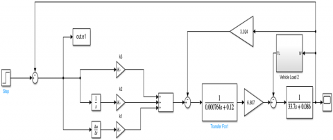
In this context, the term “Error” denotes the variance between the desired and factual speed of the electric vehicle. The Simulink diagram depicted in Figure 7 illustrates the implementation of the proportional-integral-derivative (PID) controller on the electric vehicle (EV) model.
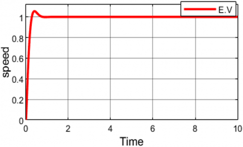
In Figure 8 evidently, the maximal velocity underwent a significant reduction and the recorded measurement approached the anticipated speed, albeit with a protracted period of ascension to attain the coveted value. Table 3 portrays the acquired outcomes of the conventional PID optimization, along with the optimal values attained for the controller.
Figure 7. Simulation model of the EV speed control
Figure 8. Output of the simulated EV using conventional PID controller (pu: per unit)
Table 3. Results of the conventional PID optimization
|
Method |
Optimum Gain Values |
M.P. (%) |
Ts (sec) |
Tr (sec) |
Steady-State Error |
|
Conventional PID |
Kp=4.34 Ki=43.0663 Kd=-0.00295 |
7.67 |
0.582 |
0.158 |
0 |
Table 4. The PSO variables
|
Values |
Variable Name |
|
|
0.4 |
Inertia |
|
|
100 |
Number of iterations |
|
|
20 |
Number of particles |
|
|
2 |
Cognitive component c1 |
|
|
2 |
Cognitive component c2 |
|
|
Lower=0.1 Upper=300 |
Kp, Ki and Kd bounds |
PID |
|
Lower=0.1 Upper=300 |
Kp, Ki and Kd bounds |
FOPID |
|
Lower=0.1 Upper=1 |
λ, and μ bounds |
|
The PSO algorithm is utilized to train a PID controller by adjusting its physical parameters in MATLAB. This involves modifying the m file in conjunction with the Simulink model, as shown in Figure 9. Through iterative experimentation and analysis of the results presented in Table 4, the aim is to improve the system’s performance by finding optimal values for the PID controller’s Kp, Ki, and Kd, which were determined to be 12.187, 130.766, and 0.0633, respectively. The results indicate significant settling time, rise time and overshoot improvements compared to the classical PID response.
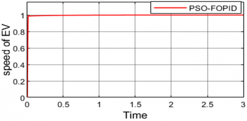
Additionally, the FOPID controller algorithm is employed for parameter tuning. The optimal values for the FOPID controller’s parameters (Kp, Ki, Kd, λ, and μ) are determined to be 112.41, 296.103, 0.6151, 0.9501, and 0.9570, respectively. The step responses of the EV speed, governed by the PSO-PID and PSO-FOPID controllers, are depicted in Figure 9 and Figure 10. The outcomes of the optimization process are tabulated in Table 5.
Upon juxtaposing the system responses, it is evident that the simulation outcomes evince a noteworthy advancement in the system response efficacy by utilizing the FOPID controller. This is evidenced by the improvement of all parameters in the system, thereby attesting to the superior performance of the proposed FOPID controller over the PID controller that employs the PSO algorithm.
In the process of training the PID controller via the GWO algorithm, the selection of GWO variables was determined through a series of iterative experiments. The objective of these experiments was to optimize system performance, as evidenced by the data presented in Table 6.
Figure 9. Step responses of the EV using PSO-PID controllers
Figure 10. Step responses of the EV using PSO-FOPID controllers
Table 5. Comparison between the proposed PID and the FOPID controllers’ results using the PSO algorithm
|
Method |
Optimum Gain Values |
M.P. (%) |
Ts (sec) |
Tr (sec) |
Steady-State Error |
|
PSO-PID |
Kp=12.187 Ki=130.766 Kd=0.0633 |
1.531 |
0.076 |
0.0539 |
0.0000513 |
|
PSO-FOPID |
Kp=112.41 Ki=296.103 Kd=0.6151 λ=0.9501 μ=0.9570 |
0.505 |
0.00955 |
0.00846 |
0.000365 |
The GWO algorithm trains a PID controller by adjusting its physical parameters, as shown in Figure 7. Through repeated experimentation and analysis of the results presented in Table 6, the goal is to improve system performance by finding optimal values for the PID controller Kp, Ki, and Kd, which are determined to be 17.132, 82.054, and 0.520, respectively. The results indicate a significant improvement in settling time, rise time and overshoot compared to the conventional PID response.
Table 6. The GWO variables
|
Values |
Variable Name |
|
|
100 |
No. of iteration |
|
|
9 |
Population size (N) |
|
|
20 |
Sample size |
|
|
0.7 |
Evaporate rate |
|
|
2 |
Scaling rate |
|
|
Lower=0.1 Upper=300 |
Kp, Ki and Kd bounds |
PID |
|
Lower=0.1 Upper=300 |
Kp, Ki and Kd bounds |
FOPID |
|
Lower=0.1 Upper=1 |
λ, and μ bounds |
|
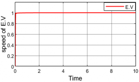
In addition, a FOPID control algorithm is used to adjust the parameters. The optimal values for the parameters of the FOPID controller (Kp, Ki, Kd, λ, and μ) were determined to be 25.982, 178.78, 4.7037, 0.9064, and 0.2758, respectively. The step responses to the EV velocity, governed by the GWO-PID and GWO-FOPID controllers, are depicted in Figure 11 and Figure 12. The results of the improvement process are tabulated in Table 7.
Figure 11. Step responses of the EV using GWO-PID controllers
Figure 12. Step responses of the EV using GWO-FOPID controllers
When comparing the system responses, it is clear that the simulation results show a significant progression in the effectiveness of the system response through the use of the FOPID controller. This is evidenced by the optimization of all parameters in the system and thus attests to the superior performance of the proposed FOPID controller over the PID controller using the GWO algorithm. It is evident through the comparison as in Table 7 that the FOPID-GWO control unit is superior to the FOPID-PSO control unit in terms of Steady-state error and overshoot.
Table 7. Comparison between the proposed PID and the FOPID controllers’ results using the GWO algorithm
|
Method |
Optimum Gain Values |
M.P. (%) |
Ts (sec) |
Tr (sec) |
Steady-State Error |
|
GWO-PID |
Kp=17.132 Ki=82.054 Kd=0.520 |
0.505 |
0.548 |
0.144 |
0.00065 |
|
GWO-FOPID |
Kp=25.982 Ki=178.78 Kd=4.7037 λ=0.9064 μ=0.2758 |
0.257 |
0.0438 |
0.0235 |
0.00025 |
The research aimed to optimize the FOPID controller for EVs speed control utilizing the GWO and PSO algorithms. The primary objective was to minimize the ITAE objective function, a metric assessing the controller’s ability to accurately track the desired speed while minimizing error accumulation over time. Various performance metrics, including transient response, frequency response, settling time, rising time, and ITAE, were meticulously analyzed to gauge the effectiveness of the proposed GWO-FOPID controller in comparison to other controllers such as GWO-PID, PSO-PID, and PSO-FOPID.
The results unequivocally demonstrated the superiority of the GWO-FOPID controller over its counterparts. This finding holds significant implications for the design of electric vehicles, suggesting that employing the GWO-FOPID controller could substantially enhance the precision and efficiency of speed regulation in EVs. Beyond the realm of electric vehicles, these results also contribute valuable insights to the broader field of control systems, emphasizing the potential of intelligent optimization algorithms in refining controller performance across various applications.
In terms of future research directions, a more targeted approach could involve exploring specific aspects of the controller that could be further improved. For instance, investigating methods to enhance the controller’s adaptability to varying driving conditions or evaluating its robustness against unexpected disturbances could be valuable areas of focus. Additionally, delving into advanced algorithms or hybrid approaches that combine the strengths of different optimization techniques might lead to even more optimized controllers.
Acknowledging the limitations of the study is crucial for a comprehensive understanding. For instance, the study might have specific constraints related to the chosen optimization algorithms or the complexity of the EV model. Addressing these limitations in future research endeavors could provide a more nuanced perspective on the proposed controller’s applicability and potential areas of refinement. By taking these factors into account, future studies can build upon these findings to develop even more sophisticated and effective control systems for electric vehicles and related applications.
[1] Chen, L., Sun, X.D., Jiang, H.B., Xu, X. (2014). A high-performance control method of constant V/f-controlled induction motor drives for electric vehicles. Mathematical Problems in Engineering, 2014. https://doi.org/10.1155/2014/386174
[2] Li, X.Y., Tian, W., Gao, X.N., Yang, Q.F., Kennel, R. (2021). A generalized observer-based robust predictive current control strategy for PMSM drive system. IEEE Transactions on Industrial Electronics, 69(2): 1322-1332. https://doi.org/10.1109/TIE.2021.3062271
[3] Morimoto, S. (2007). Trend of permanent magnet synchronous machines. IEEJ Transactions on Electrical and Electronic Engineering, 2(2): 101-108. https://doi.org/10.1002/tee.20116
[4] Yadav, D., Verma, A. (2018). Comperative performance analysis of PMSM drive using MPSO and ACO techniques. International Journal of Power Electronics and Drive System, 9(4): 1510-1522. https://doi.org/10.11591/ijpeds.v9.i4.pp1510-1522
[5] Garcia-Gonzalo, E., Fernández-Martínez, J.L. (2012). A brief historical review of particle swarm optimization (PSO). Journal of Bioinformatics and Intelligent Control, 1(1): 3-16. https://doi.org/10.1166/jbic.2012.1002
[6] Raisemche, A., Boukhnifer, M., Larouci, C., Diallo, D. (2013). Two active fault-tolerant control schemes of induction-motor drive in EV or HEV. IEEE Transactions on Vehicular Technology, 63(1): 19-29. https://doi.org/10.1109/TVT.2013.2272182
[7] Merzoug, M.S., Naceri, F. (2008). Comparison of field-oriented control and direct torque control for permanent magnet synchronous motor (PMSM), International Journal of Electrical and Computer Engineering, 2(9), 1797–1802.
[8] Munoz-Hernandez, G.A., Mino-Aguilar, G., Guerrero-Castellanos, J.F., Peralta-Sanchez, E. (2020). Fractional order PI-based control applied to the traction system of an electric vehicle (EV). Applied Sciences, 10(1): 364. https://doi.org/10.3390/app10010364
[9] George, M.A., Kamat, D.V., Kurian, C.P. (2022). Electric vehicle speed tracking control using an ANFIS-based fractional order PID controller. Journal of King Saud University-Engineering Sciences. https://doi.org/10.1016/j.jksues.2022.01.001
[10] Babaei, F., Lashkari, Z.B., Safari, A., Farrokhifar, M., Salehi, J. (2020). Salp swarm algorithm‐based fractional‐order PID controller for LFC systems in the presence of delayed EV aggregators. IET Electrical Systems in Transportation, 10(3): 259-267. https://doi.org/10.1049/iet-est.2019.0076
[11] Sebastian, A., Karbasizadeh, N., Saikumar, N., HosseinNia, S.H. (2021). Augmented fractional-order reset control: Application in precision mechatronics. In 2021 IEEE/ASME International Conference on Advanced Intelligent Mechatronics (AIM), pp. 231-238. https://doi.org/10.1109/AIM46487.2021.9517368
[12] Ibraheem, I.K., Ibraheem, G.A. (2016). Motion control of an autonomous mobile robot using modified particle swarm optimization based fractional order PID controller. Engineering and Technology Journal, 34(13A): 2406-2419. https://doi.org/10.30684/etj.34.13A.4
[13] An, W.P., Wang, H.Q., Sun, Q.Y., Xu, J., Dai, Q.H., Zhang, L. (2018). A PID controller approach for stochastic optimization of deep networks. In 2018 IEEE/CVF Conference on Computer Vision and Pattern Recognition (CVPR), Salt Lake City, UT, USA, pp. 8522-8531. https://doi.org/10.1109/CVPR.2018.00889
[14] Jassim, A.A., Karam, E.H., Ali, M.M.E. (2023). Design of optimal PID controller for electric vehicle based on particle swarm and multi-verse optimization algorithms. Engineering and Technology Journal, 41(2): 446-455. https://doi.org/10.30684/etj.2023.135587.1279
[15] Khooban, M.H., ShaSadeghi, M., Niknam, T., Blaabjerg, F. (2017). Analysis, control and design of speed control of electric vehicles delayed model: Multi‐objective fuzzy fractional‐order controller. IET Science, Measurement & Technology, 11(3): 249-261. https://doi.org/10.1049/iet-smt.2016.0277
[16] Veeresh, M.Y., Reddy, V.N.B., Kiranmayi, R. (2022). Modeling and analysis of time response parameters of a PMSM-based electric vehicle with PI and PID controllers. Engineering, Technology & Applied Science Research, 12(6): 9737-9741. https://doi.org/10.48084/etasr.5321
[17] Singh, B., Singh, B.P., Dwivedi, S. (2006). DSP based implementation of hybrid speed controller for vector controlled permanent magnet synchronous motor drive. In 2006 IEEE International Symposium on Industrial Electronics, 3: 2235-2241. https://doi.org/10.1109/ISIE.2006.295920
[18] Karteek, Y.V.P., Kumar, N.P. (2016). Transfer function model based analysis of permanent magnet synchronous motor with controllers. International Journal of Innovative Research in Electrical, Electronics, Instrumentation and Control Engineering, 4(11): 8-14. https://doi.org/10.17148/IJIREEICE.2016.41102
[19] Kuntanapreeda, S. (2014). Traction control of electric vehicles using sliding-mode controller with tractive force observer. International Journal of Vehicular Technology, 2014: 1-9. https://doi.org/10.1155/2014/829097
[20] Li, J.Y., Wu, L., Wen, G.Q., Li, Z. (2019). Exclusive feature selection and multi-view learning for Alzheimer’s disease. Journal of Visual Communication and Image Representation, 64: 102605. https://doi.org/10.1016/j.jvcir.2019.102605
[21] Ibrahim, E.K., Issa, A.H., Gitaffa, S.A. (2022). Optimization and performance analysis of fractional order PID controller for DC motor speed control. Journal Européen des Systémes Automatisés, 55(6): 741-748. https://doi.org/10.18280/jesa.550605
[22] Mirjalili, S., Mirjalili, S.M., Lewis, A. (2014). Grey wolf optimizer. Advances in Engineering Software, 69: 46-61. https://doi.org/10.1016/j.advengsoft.2013.12.007
[23] Ahmed, A., Gupta, R., Parmar, G. (2018). GWO/PID approach for optimal control of DC motor. In 2018 5th International Conference on Signal Processing and Integrated Networks (SPIN), Noida, India, pp. 181-186. https://doi.org/10.1109/SPIN.2018.8474105
[24] Guha, D., Roy, P.K., Banerjee, S. (2016). Load frequency control of large scale power system using quasi-oppositional grey wolf optimization algorithm. Engineering Science and Technology, an International Journal, 19(4): 1693-1713. https://doi.org/10.1016/j.jestch.2016.07.004
[25] Al-Khazraji, H. (2022). Optimal design of a proportional-derivative state feedback controller based on meta-heuristic optimization for a quarter car suspension system. Mathematical Modelling of Engineering Problems, 9(2): 437-442. https://doi.org/10.18280/mmep.090219
[26] Reznik, L. (1997). Fuzzy Controllers. Newnes. An imprint of Butterworth.
[27] Mahfouz, A.A., Mamdouh, W.M. (2012). Intelligent DTC for PMSM drive using ANFIS technique. International Journal of Engineering Science and Technology, 4(3): 1208-1222.
[28] Azzawi, H.A., Ameen, N.M., Gitaffa, S.A. (2023). Comparative performance evaluation of swarm intelligence-based FOPID controllers for PMSM speed control. Journal Européen des Systèmes Automatisés, 56(3): 475-482. https://doi.org/10.18280/jesa.560315