Marco Nicola Mastrone![]() | Franco Concli*
| Franco Concli*![]()
© 2023 IIETA. This article is published by IIETA and is licensed under the CC BY 4.0 license (http://creativecommons.org/licenses/by/4.0/).
OPEN ACCESS
Aeration refers to the air entrapment in a second fluid. In mechanical transmissions (as gearboxes and turbines) it affects the reliability of the system by reducing its performance and leading to early failure of the components. Air bubbles decrease the effectiveness of the lubricant by directly impacting on its heat transfer capabilities. The analysis of aeration in gearboxes is traditionally based on experiments, which require niche equipment for its evaluation. The last decade has been characterized by huge improvements in the field of numerical calculus and computer technology. These led to the implementation of sophisticated virtual models capable of reproducing complex multiphase operating conditions. In the present work, Computational Fluid Dynamics (CFD) was exploited to study the effect of a new solver (implemented in the OpenFOAM® framework) that considers aeration. The solver was used for the simulation of a real gearbox in which aeration was observed. The results were analysed qualitatively in terms of amount of increase of the lubricant mixture volume, and quantitatively in terms of power dissipation estimation. The promising outcomes of this analysis suggests that this tool can be possibly exploited to have a deeper insight in the aeration phenomenon.
CFD, aeration, multiphase simulation, OpenFOAM
Simulation tools are nowadays used both in academia to perform research activities and in industries for the development of new products. The benefits in terms of cost and time reduction with respect to physical prototypes make these tools particularly appreciated by engineers. The virtual modeling phase requires a deep knowledge of the physics involved in the investigation in order to make the correct assumptions and to apply the proper boundary conditions. Multiphase problems are usually complex to be handled numerically because of the necessity to consider more fluids at the same time and to manage the interface among them. Being able to treat them correctly is fundamental to study typical engineering applications as hydraulic systems and lubrication of components. Physical processes as cavitation and aeration cannot be modelled with default multiphase solvers. These usually cause excessive noise, premature failures, and efficiency reductions. The inclusion of such phenomena in the virtual model requires to integrate the code by adding a source term in the conservation equation that accounts for the multiphase problem.
In particular, aeration has still not been considered in the numerical analysis of mechanical systems as geared transmissions. On the other hand, several works dealing with multiphase solvers, both mesh-based [1-18] and mesh-less [19-24], and cavitation simulations [25-30] can be found in literature. Pioneering studies on aeration in mechanical components can be found in the study [31], where the authors analysed the aeration in tapered roller bearings with experimental and numerical investigations. The adoption of a solver for capable of considering aeration can bring significant benefits in the numerical analysis of this phenomenon, that diminishes the performance of the lubricant as a consequence of the lower heat transfer capabilities and efficiency reduction.
Since the experimental investigation of aeration in gearboxes requires advanced measuring techniques [32, 33], numerical methods could offer a good solution to analyze this problem with simulation codes. Cerne et al. [34] introduced an interface tracking algorithm based on a two-fluid model formulation [35]. An extension of the previous model for three fluids was proposed by Yan and Che [36]. A combination of Eulerian approach and Volume of Fluid (VOF) was tested by Wardle and Weller [37]. Ma et al. [38] reformulated the source term proposed by Sene [39] by including the turbulent intensity in their model and tested it on different test cases [40-42]. Several investigations have considered plunging jet [43-46] because of the typical air bubbles generation at free surface. In this work, (an extension of the results presented at a conference [47]) a solver that considers aeration implemented in OpenFOAM® [48] is applied to a gearbox to predict the level of aeration based on the foaming effects. The results indicate that this solver may represent a good choice to study the aeration phenomenon numerically and may be a good solution if the real prototypes do not allow an easy experimental analysis.
2.1 Mathematical description
For the analyzed case, the simulations were considered isothermal. Therefore, the energy equation was not activated, and the conservation equations of mass and momentum were solved by the CFD code (Reynolds Averaged Navier-Stokes - RANS for incompressible not-stationary flow):
$\rho \frac{\partial\left\langle\boldsymbol{u}_{\boldsymbol{i}}\right\rangle}{\partial x_i}=0$ (1)
$\rho \frac{\partial\left\langle\boldsymbol{u}_i\right\rangle}{\partial t}+\rho \frac{\partial\left\langle\boldsymbol{u}_i\right\rangle\left\langle\boldsymbol{u}_i\right\rangle}{\partial x_j}=-\frac{\partial\langle p\rangle}{\partial x_i}+\frac{\partial}{\partial x_j}\left[\mu\left(\frac{\partial\left\langle\boldsymbol{u}_i\right\rangle}{\partial x_j}+\frac{\partial\left\langle\boldsymbol{u}_j\right\rangle}{\partial x_i}\right)\right]-\frac{\partial \tau_{i j}}{\partial x_j}$ (2)
The term τij is the unresolved term and can be written taking advantage of the eddy viscosity (μt) hypothesis:
$-\tau_{i j}=\mu_t\left(\frac{\partial\left\langle\boldsymbol{u}_{\boldsymbol{i}}\right\rangle}{\partial x_j}+\frac{\partial\left\langle\boldsymbol{u}_{\boldsymbol{j}}\right\rangle}{\partial x_i}\right)-\frac{2}{3} \delta_{i j} k$ (3)
$\mu_t=C_\mu \rho \frac{k^2}{\varepsilon}$ (4)
Turbulence is modeled according the RNG k-ε model:
$\rho \frac{\partial}{\partial t}(k)+\rho \frac{\partial}{\partial x_i}\left(k u_i\right)=\frac{\partial}{\partial x_j}\left[\alpha_k \mu_{\mathrm{eff}} \frac{\partial k}{\partial x_j}\right]+G_k+G_b-\rho \varepsilon-Y_M+S_k$ (5)
$\rho \frac{\partial}{\partial t}(\varepsilon)+\rho \frac{\partial}{\partial x_i}\left(\varepsilon u_i\right)=\frac{\partial}{\partial x_j}\left[\alpha_{\varepsilon} \mu_{\mathrm{eff}} \frac{\partial k}{\partial x_j}\right]+\frac{C_{1 \varepsilon} \varepsilon}{k}\left(G_k+C_{3 \varepsilon} G_b\right)-\frac{C_{2 \varepsilon} \rho \varepsilon^2}{k}-R_{\varepsilon}+S_{\varepsilon}$ (6)
Since these equations are valid only in monophasic simulations, a third conservation equation is added for two fluids. The VOF model [49] is used. The equation of the volumetric fraction (percentage of one fluid in every cell of the domain) is:
$\frac{\partial \alpha}{\partial t}+\nabla(\alpha \boldsymbol{u})=0$ (7)
A generic physical property $\Theta$ (like viscosity and density) of the two fluids is used to describe an equivalent fluid such that:
$\Theta_{\mathrm{eq}}=\Theta_1 \cdot \alpha+\Theta_2 \cdot(1-\alpha)$ (8)
The value of α can assume values between 0 and 1. In order to guarantee a bounded solution, the compressive scheme MULES (Multidimensional Universal Limiter with Explicit Solution) [50] was used. The MULES improves the interface resolution by the addition of the relative velocity uc that, by acting perpendicularly to the interface, estimates the relative velocity between fluids. The equation of α becomes:
$\frac{\partial \alpha}{\partial t}+\nabla(\alpha \boldsymbol{u})+\nabla\left(\boldsymbol{u}_c \alpha(1-\alpha)\right)=0$ (9)
The further addition of a source term to the right part of the equation (Sg) permits to include also physical phenomena as aeration and cavitation:
$\frac{\partial \alpha}{\partial t}+\nabla(\alpha \boldsymbol{u})+\nabla\left(\boldsymbol{u}_c \alpha(1-\alpha)\right)=S_g$ (10)
In this work, aeration is modelled according to Hirt [51]. In this model, the source term is given as an explicit term in the α equation:
$S_g=C_{a i r} A_S \sqrt{2 \frac{P_t-P_d}{\rho}}$ (11)
where, Cair is a calibration parameter, AS the free surface area at each cell, ρ is the fluid density, and Pt (turbulent forces) and Pd(stabilizing forces) are given by:
$\boldsymbol{P}_{\boldsymbol{t}}=\rho k$ (12)
$\boldsymbol{P}_{\boldsymbol{d}}=\rho \boldsymbol{g}_{\boldsymbol{n}} L_T+\frac{\boldsymbol{\sigma}}{L_T}$ (13)
where, gn is the component of the gravity normal to the free surface, σ is the surface tension, and LT is the turbulence characteristic length scale, expressed as:
$L_T=C_\mu \cdot \sqrt{\frac{3}{2}} \frac{k^{\frac{3}{2}}}{\varepsilon}$ (14)
According to Eq. (11), when Pt>Pd an air volume is added to the cell in question. The coefficient of proportionality Cair in the equation of the source term is set to 0.5. This value was used by Hirt for many test cases, and he concluded that this value can be reasonable for most of the applications, as on average it can be assumed that air will be entrapped over about half the surface area.
2.2 Solver settings
The PIMPLE algorithm was adopted to solve the transient simulations. Two correctors of the pressure equation were imposed to maintain the stability of the solution. A convergence criterion of 1e-6 was imposed to all field’s variables. The PCG (Preconditioned Conjugate Gradient) solver was used for the pressure. The velocity was solved with the PBiCG (Stabilized preconditioned bi-conjugate gradient). The timestep was set to achieve a maximum courant number of 1. The time derivative was discretized with the first order implicit Euler scheme, while the velocity with the second order linearUpwind scheme and the convection of the volumetric fraction with the vanLeer scheme. The turbulence quantities were discretized with the second order linearUpwind scheme.
In order to study the new solver that considers aeration, firstly, a simple benchmark case consisting in a vertical plunging jet is considered; secondly, a gearbox is analysed with a standard multiphase solver and the new implemented one to investigate the capability to estimate the aeration level. Lastly, the velocity field of a tapered roller bearing was compared with experimental measurements with both solvers. The results indicate that a better physical representation can be obtained with the new solver capable of modelling the entrapment of air in liquid phase.
3.1 Vertical plunging jet
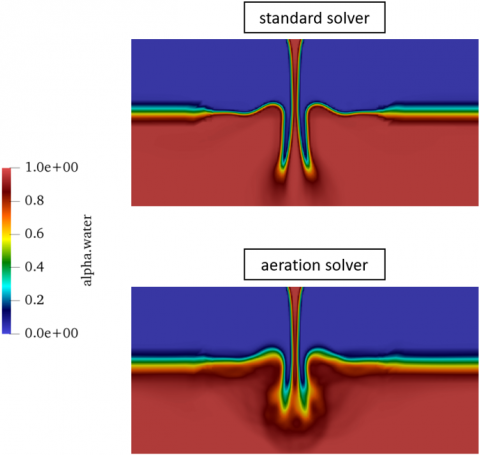
The gradients of velocity that originate at the free surface causes in most cases aeration. For this reason, a vertical plunging jet was considered the most appropriate test case to validate the new numerical solver. The problem consists of a square box with dimensions 600×600 mm2 filled with water for an area of 500×500 mm2. The domain is discretized with quad elements. The water jet has an ejection velocity of 0.4 m/s.
In Figure 1, it is possible to appreciate the difference of the flow characteristics between a standard multiphase solver and the one that considers aeration. While on the left-hand side the interface between the two fluids is sharp (standard solver), on the right-hand side it appears smooth, indicating a high concentration of air in that region. The qualitative analysis based on the water fluxes suggests that this solver can model the air entrapment.
Figure 1. Detail of the free surface water-air (standard vs aeration solver)
3.2 Single rotating gear
A rotating gear is considered as a direct application of the implemented solver to quantify the level of aeration in a real operating condition. The wheel’s parameters are reported in Table 1.
Table 1. Wheel’s design parameters
|
|
Unit |
Wheel |
|
Number of teeth |
- |
24 |
|
Module |
mm |
4.5 |
|
Face width |
mm |
14.0 |
|
Pitch diameter |
mm |
109.8 |
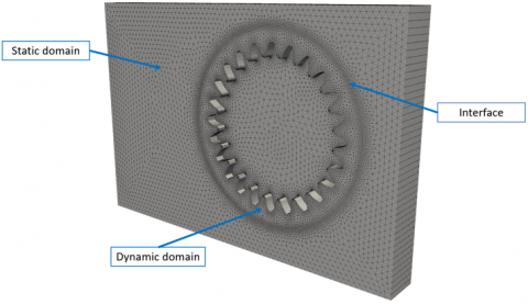
The domain was discretized with triangular prisms (Figure 2). Firstly, a 2D partition of the gearbox was meshed. The global 3D mesh was then obtained by extruding the 2D grid in the two axial directions. The sliding mesh approach was used to simulate the gear’s rotation: the region surrounded by a cylinder is assigned as “dynamic”, while the rest of the box as “static”. In this way, the dynamic cells can rotate and slide along the static cells. The definition of an interface allows the numerical connection between the two regions even in case the nodes are not conformal during the dynamic motion.
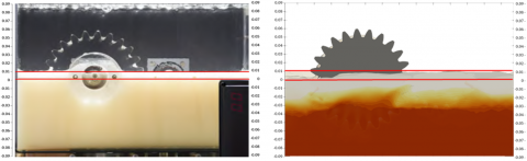
The gearbox was filled with oil at centreline level. The oil has a kinematic viscosity of $v_{40^{\circ} C}=22 \frac{mm^2}{{~s}}$ and a density of $\rho_{40^{\circ} {C}}=900 \frac{{kg}}{{m}^3}$. The gear rotates with an angular velocity of 3000 rpm. In this condition, the lubricant showed an aeration level of about 10% experimentally [52]. In order to estimate the aeration level experimentally, the wheel’s rotation was slowed down to zero so that the mixture could drop. It is expected that the level of the mixture will be higher due the air entrainment in the lubricant. Similarly to experiments, the gear’s velocity was slowed down to zero after the physical regime condition, so that the mixture could fall, and the aeration level could be estimated in the virtual model. In Figure 3 the comparison between experimental and the simulation mixture’s level is illustrated. It can be noticed that air entrapment at free surface is predicted by the simulation in form of foaming effects, resulting in a comparable aeration level with respect to experiments. The values of α have been divided in 3 ranges: from 0 to 0.33 (pure oil), from 0.33 to 0.66 (oil and foaming effects), from 0.66 to 1 (pure air). The plotted lubricant level ranges therefore from 0 to 0.66 in order to account for the possible foaming effects.
Figure 2. Numerical mesh. The static and the dynamic mesh are connected by an interface
Figure 3. Aeration level: Experimental-simulation comparison
The analysis on the power dissipation showed that aeration promotes an increase of the losses, in accordance with literature [53-55]. In particular, at the investigated operating condition the aerated configuration exhibited about 5% increase in the power losses with respect to the non-aerated configuration. This is due to the increasing energy at the interface between air bubbles and lubricant that promotes a higher power dissipation.
3.3 Tapered roller bearing
The default and the new solver were used to study the velocity field of a tapered roller bearing 32312-A (whose design can be found in the study [56]) and the results compared with experimental data. In order to enable to optical access for the PIV measurements, a sapphire outer ring was manufactured instead of a classic steel component. By doing so, a laser light could access the bearing radially and the images could be acquired by two cameras. The bearing was completely submerged by the lubricant, which was seeded with fluorescent polystyrene particles. The target domain of the measurements lies in the plane region between two rollers.
The cyclic symmetry of the bearing was exploited, thus only a sector was modelled. A fully hexahedral mesh with about 800k cells was generated (Figure 4).
Figure 4. Numerical mesh with a detailed view near the roller
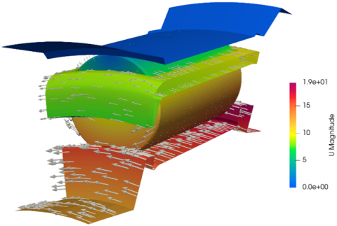
A rigid mesh motion was applied to the whole domain. The speed of the rings was defined by adjusting the velocities in the rotating reference frame, while the rotation of the roller around its own axis was considered by implementing a dedicated boundary condition. In Figure 5 the velocity contour and vectors representing the kinematics of the different components is reported.
Figure 5. Velocity contour and vectors of the different patches
The rotational speed of the cage is 2000 rpm. At this velocity, experimentally it was observed that aeration occurs. The lubricant has a kinematic viscosity of $v_{25^{\circ} C}=21 \frac{mm^2}{{~s}}$ and a density of $\rho_{25^{\circ} {C}}=870 \frac{{kg}}{{m}^3}$. In Figure 6 the comparison between PIV measurements and numerical results (no aeration and aeration solver) is presented.
Figure 6. PIV vs CFD (no aeration) vs CFD (aeration) velocity field
From experiments, a high velocity region on the right part of the target domain is present. While the simulation with the solver that does not consider aeration leads to a high velocity region on the left part of the target domain in contrast with experiments, the solver that considers aeration provides results in agreement with measurements. The default solver is not capable of reproducing the aeration phenomenon and the related flow field correctly.
Nowadays, the design of mechanical systems is increasingly accompanied by numerical studies to have a deeper insight on the systems’ behaviour. In this sense, CFD codes can be used to analyse multiphase operating conditions, which usually require specific prototypes and equipment to obtain data. In this work, the opensource software OpenFOAM® was used to implement a solver capable of modelling the aeration phenomenon. The preliminary test on a vertical plunging jet allowed to study a simple case in which aeration usually occurs. The good physical representation of this problem suggested the extension of the application of this solver to mechanical systems. Indeed, a single gear rotating at high speed was simulated, and the results were compared with experimental data in terms of aeration level. The qualitative analysis shows that air is added at free surface, resulting in an increase level of the mixture’s volume due to the foaming effects given by the air entrapment. Moreover, the solver was exploited to study a tapered roller bearing, demonstrating its capability to reproduce the experimentally measured velocity field with respect to the default solver, which led to completely wrong predictions. The good agreement of the new implemented solver with respect to experiments indicate this tool being appropriate for an estimation of fluid’s comportment and the efficiency of the considered system in case of aeration.
[1] Burberi, E., Fondelli, T., Andreini, A., Facchini, B., Cipolla, L. (2016). CFD simulations of a meshing gear pair. In Turbo Expo: Power for Land, Sea, and Air, 49781: V05AT15A024. https://doi.org/10.1115/GT2016-57454
[2] Mastrone, M.N., Hartono, E.A., Chernoray, V., Concli, F. (2020). Oil distribution and churning losses of gearboxes: Experimental and numerical analysis. Tribology International, 151: 106496. https://doi.org/10.1016/j.triboint.2020.106496
[3] Frosina, E., Senatore, A., Buono, D., Manganelli, M.U., Olivetti, M. (2014). A tridimensional CFD analysis of the oil pump of an high performance motorbike engine. Energy Procedia, 45: 938-948. https://doi.org/10.1016/j.egypro.2014.01.099
[4] Ferrari, C., Marani, P. (2016). Study of air inclusion in lubrication system of CVT gearbox transmission with biphasic CFD simulation. In Fluid Power Systems Technology, 50060: V001T01A031. https://doi.org/10.1115/FPMC2016-1767
[5] Santra, T.S., Raju, K., Deshmukh, R., Gopinathan, N., Paradarami, U., Agrawal, A. (2019). Prediction of oil flow inside tractor transmission for splash type lubrication (No. 2019-26-0082). SAE Technical Paper. https://doi.org/10.4271/2019-26-0082
[6] Huang, S., Wei, Y., Guo, C., Kang, W. (2019). Numerical simulation and performance prediction of centrifugal pump’s full flow field based on OpenFOAM. Processes, 7(9): 605. https://doi.org/10.3390/pr7090605
[7] Mastrone, M.N., Concli, F. (2021). CFD simulation of grease lubrication: Analysis of the power losses and lubricant flows inside a back-to-back test rig gearbox. Journal of Non-Newtonian Fluid Mechanics, 297: 104652. https://doi.org/10.1016/j.jnnfm.2021.104652
[8] Mastrone, M.N., Concli, F. (2021). Power losses of spiral bevel gears: An analysis based on computational fluid dynamics. Frontiers in Mechanical Engineering, 7: 655266. https://doi.org/10.3389/fmech.2021.655266
[9] Petit, O., Nilsson, H. (2013). Numerical investigations of unsteady flow in a centrifugal pump with a vaned diffuser. International Journal of Rotating Machinery, 2013: 961580. https://doi.org/10.1155/2013/961580
[10] Hildebrand, L., Dangl, F., Sedlmair, M., Lohner, T., Stahl, K. (2022). CFD analysis on the oil flow of a gear stage with guide plate. Forschung im Ingenieurwesen, 86(3): 395-408. https://doi.org/10.1007/s10010-021-00523-5
[11] Concli, F., Schaefer, C.T., Bohnert, C. (2019). Innovative strategies for bearing lubrication simulations. Preprints.org 2019: 2019100218. https://doi.org/10.20944/preprints201910.0218.v1
[12] Liu, H., Jurkschat, T., Lohner, T., Stahl, K. (2017). Determination of oil distribution and churning power loss of gearboxes by finite volume CFD method. Tribology International, 109: 346-354. https://doi.org/10.1016/j.triboint.2016.12.042
[13] Peng, Q., Zhou, C., Gui, L., Fan, Z. (2019). Investigation of the lubrication system in a vehicle axle: Optimization and experimental validation. Proceedings of the Institution of Mechanical Engineers, Part D: Journal of Automobile Engineering, 233(8): 2096-2107. https://doi.org/10.1177/0954407018766130
[14] Dai, Y., Jia, J., Ouyang, B., Bian, J. (2020). Determination of an optimal oil jet nozzle layout for helical gear lubrication: Mathematical modeling, numerical simulation, and experimental validation. Complexity, 2020: 2187027. https://doi.org/10.1155/2020/2187027
[15] Peng, Q., Gui, L., Fan, Z. (2018). Numerical and experimental investigation of splashing oil flow in a hypoid gearbox. Engineering Applications of Computational Fluid Mechanics, 12(1): 324-333. https://doi.org/10.1080/19942060.2018.1432506
[16] Lu, F., Wang, M., Bao, H., Huang, W., Zhu, R. (2022). Churning power loss of the intermediate gearbox in a helicopter under splash lubrication. Proceedings of the Institution of Mechanical Engineers, Part J: Journal of Engineering Tribology, 236(1): 49-58. https://doi.org/10.1177/13506501211010030
[17] Lu, F., Wang, M., Pan, W., Bao, H., Ge, W. (2020). CFD-based investigation of lubrication and temperature characteristics of an intermediate gearbox with splash lubrication. Applied Sciences, 11(1): 352. https://doi.org/10.3390/app11010352
[18] Mastrone, M.N., Concli, F. (2022). A multi domain modeling approach for the CFD simulation of multi-stage gearboxes. Energies, 15(3): 837. https://doi.org/10.3390/en15030837
[19] Deng, X., Wang, S., Wang, S., Wang, J., Liu, Y., Dou, Y., He, G., Qian, L. (2020). Lubrication mechanism in gearbox of high-speed railway trains. Journal of Advanced Mechanical Design, Systems, and Manufacturing, 14(4): JAMDSM0054-JAMDSM0054. https://doi.org/10.1299/jamdsm.2020jamdsm0054
[20] Deng, X., Wang, S., Hammi, Y., Qian, L., Liu, Y. (2020). A combined experimental and computational study of lubrication mechanism of high precision reducer adopting a worm gear drive with complicated space surface contact. Tribology International, 146: 106261. https://doi.org/10.1016/j.triboint.2020.106261
[21] Morhard, B., Schweigert, D., Mileti, M., Sedlmair, M., Lohner, T., Stahl, K. (2020). Efficient lubrication of a high-speed electromechanical powertrain with holistic thermal management. Forschung im Ingenieurwesen. https://doi.org/10.1007/s10010-020-00423-0
[22] Ji, Z., Stanic, M., Hartono, E.A., Chernoray, V. (2018). Numerical simulations of oil flow inside a gearbox by Smoothed Particle Hydrodynamics (SPH) method. Tribology International, 127: 47-58. https://doi.org/10.1016/j.triboint.2018.05.034
[23] Legrady, B., Taesch, M., Tschirschnitz, G., Mieth, C.F. (2021). Prediction of churning losses in an industrial gear box with spiral bevel gears using the smoothed particle hydrodynamic method. Forsch Ingenieurwes, 86(2022): 379–388. https://doi.org/10.1007/s10010-021-00514-6
[24] Liu, H., Arfaoui, G., Stanic, M., Montigny, L., Jurkschat, T., Lohner, T., Stahl, K. (2019). Numerical modelling of oil distribution and churning gear power losses of gearboxes by smoothed particle hydrodynamics. Proceedings of the Institution of Mechanical Engineers, Part J: Journal of Engineering Tribology, 233(1): 74-86. https://doi.org/10.1177/1350650118760626
[25] Močilan, M., Husár, Š., Labaj, J., Žmindák, M. (2017). Non-stationary CFD simulation of a gear pump. Procedia Engineering, 177: 532-539. https://doi.org/10.1016/j.proeng.2017.02.257
[26] Gao, G., Yin, Z., Jiang, D., Zhang, X. (2014). Numerical analysis of plain journal bearing under hydrodynamic lubrication by water. Tribology International, 75: 31-38. https://doi.org/10.1016/j.triboint.2014.03.009
[27] Sawicki, J.T., Rao, T.V.V.L.N. (2004). Cavitation effects on the stability of a submerged journal bearing. International Journal of Rotating Machinery, 10(3): 227-232. https://doi.org/10.1155/S1023621X04000247
[28] Mastrone, M.N., Concli, F. (2021). CFD simulations of gearboxes: implementation of a mesh clustering algorithm for efficient simulations of complex system’s architectures. International Journal of Mechanical and Materials Engineering, 16: 1-19. https://doi.org/10.1186/s40712-021-00134-6
[29] Riedel, M., Schmidt, M., Stücke, P. (2013). Numerical investigation of cavitation flow in journal bearing geometry. In EPJ Web of Conferences, 45: 01081. https://doi.org/10.1051/epjconf/20134501081
[30] Mastrone, M.N., Concli, F. (2021). Development of a mesh clustering algorithm aimed at reducing the computational effort of gearboxes’ CFD simulations. Boundary Elements and other Mesh Reduction Methods XLIV, 131: 59-69.
[31] Maccioni, L., Chernoray, V.G., Mastrone, M.N., Bohnert, C., Concli, F. (2022). Study of the impact of aeration on the lubricant behavior in a tapered roller bearing: Innovative numerical modelling and validation via particle image velocimetry. Tribology International, 165: 107301. https://doi.org/10.1016/j.triboint.2021.107301
[32] Borges, J.E., Pereira, N.H., Matos, J., Frizell, K.H. (2010). Performance of a combined three-hole conductivity probe for void fraction and velocity measurement in air–water flows. Experiments in Fluids, 48: 17-31. https://doi.org/10.1007/s00348-009-0699-1
[33] Leandro, J., Bung, D.B., Carvalho, R. (2014). Measuring void fraction and velocity fields of a stepped spillway for skimming flow using non-intrusive methods. Experiments in Fluids, 55: 1-17. https://doi.org/10.1007/s00348-014-1732-6
[34] Cerne, G., Petelin, S., Tiselj, I. (2001). Coupling of the interface tracking and the two-fluid models for the simulation of incompressible two-phase flow. Journal of Computational Physics, 171(2): 776-804. https://doi.org/10.1006/jcph.2001.6810
[35] Drew, D., Passman, S. (1998). Theory of Multicomponents Fluids. New York, USA: Springer.
[36] Yan, K., Che, D. (2010). A coupled model for simulation of the gas–liquid two-phase flow with complex flow patterns. International Journal of Multiphase Flow, 36(4): 333-348. https://doi.org/10.1016/j.ijmultiphaseflow.2009.11.007
[37] Wardle, K.E., Weller, H.G. (2013). Hybrid multiphase CFD solver for coupled dispersed/segregated flows in liquid-liquid extraction. International Journal of Chemical Engineering, 2013: 128936. https://doi.org/10.1155/2013/128936
[38] Ma, J., Oberai, A.A., Drew, D.A., Lahey Jr, R.T., Moraga, F.J. (2010). A quantitative sub-grid air entrainment model for bubbly flows–plunging jets. Computers & Fluids, 39(1): 77-86. https://doi.org/10.1016/j.compfluid.2009.07.004
[39] Sene, K.J. (1988). Air entrainment by plunging jets. Chemical Engineering Science, 43(10): 2615-2623. https://doi.org/10.1016/0009-2509(88)80005-8
[40] Ma, J., Oberai, A.A., Lahey, R.T., Drew, D.A. (2011). Modeling air entrainment and transport in a hydraulic jump using two-fluid RANS and DES turbulence models. Heat and Mass Transfer, 47: 911-919. https://doi.org/10.1007/s00231-011-0867-8
[41] Ma, J., Oberai, A.A., Drew, D.A., Lahey Jr, R.T., Hyman, M.C. (2011). A comprehensive sub-grid air entrainment model for RaNS modeling of free-surface bubbly flows. The Journal of Computational Multiphase Flows, 3(1): 41-56. https://doi.org/10.1260/1757-482X.3.1.41
[42] Ma, J., Oberai, A.A., Hyman, M.C., Drew, D.A., Lahey Jr, R.T. (2011). Two-fluid modeling of bubbly flows around surface ships using a phenomenological subgrid air entrainment model. Computers & Fluids, 52: 50-57. https://doi.org/10.1016/j.compfluid.2011.08.015
[43] Baylar, A., Emiroglu, M.E. (2004). An experimental study of air entrainment and oxygen transfer at a water jet from a nozzle with air holes. Water Environment Research, 76(3): 231-237. https://doi.org/10.2175/106143004X141780
[44] Biń, A.K. (1993). Gas entrainment by plunging liquid jets. Chemical Engineering Science, 48(21): 3585-3630. https://doi.org/10.1016/0009-2509(93)81019-R
[45] Chanson, H., Aoki, S.I., Hoque, A. (2004). Physical modelling and similitude of air bubble entrainment at vertical circular plunging jets. Chemical Engineering Science, 59(4): 747-758. https://doi.org/10.1016/j.ces.2003.11.016
[46] Kiger, K., Duncan, J.H. (2012). Air-entrainment mechanisms in plunging jets and breaking waves. Annual Review of Fluid Mechanics, 44: 563-596. https://doi.org/10.1146/annurev-fluid-122109-160724
[47] Mastrone, M.N., Concli, F. (2021). Simulation of fluid’s aeration: implementation of a numerical model in an open source environment. Advances in Fluid Dynamics with emphasis on Multiphase and Complex Flow, 132: 27.
[48] Anon OpenFOAM. https://openfoam.org/, accessed on February 1, 2022.
[49] Hirt, C.W., Nichols, B.D. (1981). Volume of fluid (VOF) method for the dynamics of free boundaries. Journal of Computational Physics, 39(1): 201-225. https://doi.org/10.1016/0021-9991(81)90145-5
[50] Rusche, H. (2003). Computational fluid dynamics of dispersed two-phase flows at high phase fractions. Doctoral dissertation, Imperial College London, University of London.
[51] Hirt, C.W. (2003). Modeling turbulent entrainment of air at a free surface. Flow Science, Inc.
[52] Hartono, E.A. (2019). Experimental study on truck related power losses: The churning losses in a transmission model and active flow control at an a-pillar of generic truck cabin model. Chalmers University of Technology, Chalmers Tekniska Hogskola (Sweden).
[53] Neurouth, A., Changenet, C., Ville, F., Octrue, M., Tinguy, E. (2017). Experimental investigations to use splash lubrication for high-speed gears. Journal of Tribology, 139(6): 061104. https://doi.org/10.1115/1.4036447
[54] Leprince, G., Changenet, C., Ville, F., Velex, P., Jarnias, F. (2009). Influence of oil aeration on churning losses JSME 2009 Int. Motion Power Transm. Conf., pp. 463-468.
[55] LePrince, G., Changenet, C., Ville, F., Velex, P., Dufau, C., Jarnias, F. (2011). Influence of aerated lubricants on gear churning losses–an engineering model. Tribology Transactions, 54(6): 929-938. https://doi.org/10.1080/10402004.2011.597542
[56] Maccioni, L., Chernoray, V.G., Bohnert, C., Concli, F. (2022). Particle Image Velocimetry measurements inside a tapered roller bearing with an outer ring made of sapphire: Design and operation of an innovative test rig. Tribology International, 165: 107313. https://doi.org/10.1016/j.triboint.2021.107313