Ali Hammouche* | Mourad Hamimid | Abdelkader Kansab | Bachir Belmadani
© 2021 IIETA. This article is published by IIETA and is licensed under the CC BY 4.0 license (http://creativecommons.org/licenses/by/4.0/).
OPEN ACCESS
In this article, a coupled algorithm between the control volume method and the hysteresis dynamic energetic model for ferromagnetic hysteresis is presented. To illustrate the dynamic behavior of ferromagnetic materials, the quasi-static model is extended by adding two components to the applied magnetic field “Hedd”, and “Hexc”. The added fields are related to the excess losses and classical eddy losses. Thus, two new supplementary coefficients are added to the model parameters. The determination of those coefficients is attained by measuring the energy density for two distinct frequencies. This model introducing the magnetic induction as an independent variable is presented in order to be directly used in time-stepping finite volume calculations applied to the magnetic vector potential formulation. The calculated results are validated by experiences performed in an Epstein’s frame. To check the effectiveness of this model combined with the control volume method in the time domain, the obtained results are compared with experiments.
eddy current, energetic model, excess losses, ferromagnetic materials, hysteresis magnetic, magnetization, numerical electromagnetic computation
The accurate determination of hysteresis losses permits to carry out of highly efficient magnetic devices, especially in the high-frequency regime. During a time-varying field, the hysteresis loops in ferromagnetic materials are increased proportionally with the frequency and may be estimated by the integration over the curve. The good assessment of those losses requires an accurate approach to the hysteresis characteristics with the frequency regime [1]. Several approaches are proposed in order to offer an accurate representation of hysteresis loops in frequency regime [2, 3]. Among existing models, we note the Jiles-Atherton model [2-4], the Preisach model [5, 6] which are most widely used, and the energetic model proposed by Hans-Hauser [7, 8]. The Preisach model supposed the material as a group of small independently acting domains. These domains have a simple relay-like hysteresis mechanism [9].
Although the Preisach model is more accurate, its complicated mathematical formulation is the major restriction in numerical implementations. On the other hand, the modified inverse JA model is based on the magnetization through the domain wall motion with pinning effects [10]. The modified inverse JA is characterized by fewer parameters characterizing the B-H curve and its simplicity of implementation with field calculation procedure.
In recent years, a several important researches are devoted on hysteresis modeling in finite element field [11, 12], its complex mathematical formulation to solve Maxwell’s equations taking into account the B-H curve [13, 14] can lead to use a more simple numerical computation, such as the finite volume method.
In this work, an analogous way such made in [1] is employed to depict the hysteresis comportment using the energetic model (EM) [7, 8]. The EM is remodeled in frequency regime based on the statistical theory of iron losses separation developed by Bertotti in magnetic materials [15, 16]. The reformulation of EM in dynamic regime is based on the addition of two additional energies associated to the eddy and excess losses [17, 18]. In this situation two new parameters related to eddy and excess losses are introduced.
In order to determine these parameters, the volumetric energy density is measured for two arbitrary frequencies.
To test the validity of the proposed dynamic energetic model coupled with finite volume method, the obtained results are compared with measurements.
2.1 Quasi-static EM
In quasi-static regime, the magnetic field “H” compounds by three terms [7, 8]:
$H_{h y s}(B)=H_{\mathrm{d}}+\operatorname{sgn}(m) H_{\mathrm{r}}+H_{l}$ (1)
With, Hd represents the demagnetizing field corresponding to the linear material behaviour; Hr represents the reversible field depicts the nonlinear behavior of materials; Hl represents the irreversible field, corresponding the hysteresis effects.
where,
$H_{\mathrm{d}}=N_{\mathrm{e}} M_{\mathrm{s}} m$ (1a)
$H_{r}=h\left(\left((1+m)^{1+m}(1-m)^{1-m}\right)^{g / 2}-1\right)$ (1b)
$H_{l}=\delta\left(\frac{k}{\mu_{0} M_{s}}+c_{r} H_{r}\right)\left(1-\kappa \exp \left(-\frac{q}{\kappa}\left|m-m_{0}\right|\right)\right)$ (1c)
With, $\delta=\operatorname{sgn}\left(m-m_{0}\right)$.
$\kappa=2-\kappa_{0} \exp \left(\exp \left(-\frac{q}{\kappa}\left|m-m_{0}\right|\right)\right)$ (2)
The calculation procedure starts from the demagnetization state (m=0, k=1), and therefore, the relative magnetization “m” gradually increases such given in Eq. (1). The function “k” is calculated by the Eq. (2) based on the previous value “k0”.
2.2 Energetic model in dynamic regime
The principal concept of DEM is the adjustment of the energy density by adding two energies represented in excess “wexc” and eddy losses “wedd”. If the magnetic flux density waveform is assumed to be a sine wave, the total magnetic field can be consisting of three terms [19].
$H_{d y n}(B)=H_{h y s}(B)+H_{e d d}(t)+H_{e x c}(t)$ (3)
The equation of “Hhys” is similar to that given by Eq. (1), “Hexc”and “Hedd”are the magnetic fields created by excess losses and eddy currents respectively, and they are given in the magnetic material by Eq. (4) and Eq. (5):
$H_{e d d}(t)=k_{e d d} \frac{\Delta m}{\Delta t}$ (4)
$H_{e x c}(t)=k_{e x c}\left(\frac{\Delta m}{\Delta t}\right)^{1 / 2}$ (5)
The resulting magnetic field in frequency regime is given as:
$H_{d y n}(B)=H_{h y s t}(B)+\left(k_{e d d} \frac{\Delta m}{\Delta t}+k_{\operatorname{exc}}\left(\frac{\Delta m}{\Delta t}\right)^{1 / 2}\right)$ (6)
“kedd” and “kexc” represent the new factors of the frequency regime associated with the geometrical and physicals properties of materials [2-20]. Finally, the dynamic energetic model is characterized by nine parameters, seven of them are identified in quasi-static regime “kedd” and “kexc” are identified in dynamic regime.
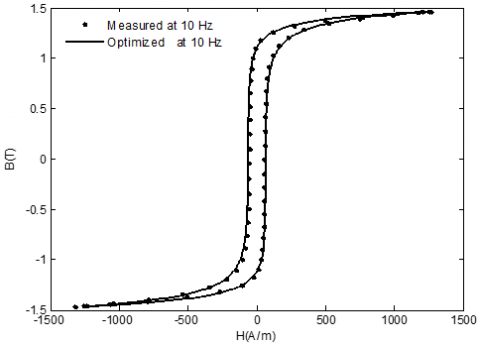
The hysteresis loops optimized and measured are plotted in Figure 1. The optimized one is calculated using EM with the parameters extracted in the case of the quasi-static regime and they are shown in Table 1. These parameters are identified from the measured hysteresis loop at low frequency of 10 Hz, by using a stochastic algorithm called simulated annealing [21]. This algorithm is implemented in MATLAB software in such a way as to achieve the best accordance between measured values “Hmeasured” and the corresponding values of optimized magnetic field “Hmodelled”. The best agreement is achieved when the minimum of used objective function (7) is found for the selected parameters.
Error $=\frac{\sqrt{\sum_{i}^{N}\left(H_{\text {measured }}^{i}-H_{\text {optimied }}^{i}\right)^{2}}}{N}$ (7)
Table 1. Parameters of energetic model in quasi-static regime
|
EM parameters |
Modelled values |
|
Ne: demagnetization coefficient |
1.58×10⁻⁷ |
|
Ms: saturation magnetization |
1.27×10⁶ |
|
h: associate with the saturation filed and anisotropy |
4.93 |
|
g: related the saturation filed and anisotropy |
9.51 |
|
k: depends on the wall displacements |
92.12 |
|
q: pinning place density |
12.40 |
|
cr: particle geometries |
0.83 |
Figure 1. Optimized and Measured hysteresis loops at 10 Hz
To obtain the coefficients “kedd” and “kexc” linked to the dynamic regime, we must solve the equations system given by (8). By measuring the energy density for two distinct frequencies (f=50Hz and f=100Hz), and Bsat=1.4T. The new dynamic coefficients obtained are illustrated in Table 2.
$\left(w_{T \alpha y}\right)_{f 1}-w_{T}=k_{e d k}\left(\int \frac{\Delta m}{\Delta t} d m\right)_{f 1}+k_{\operatorname{exc}}\left(\int\left(\frac{\Delta m}{\Delta t}\right)^{1 / 2} d m\right)_{f 1}$
$\left(w_{T \alpha y}\right)_{f 2}-w_{T}=k_{e d d}\left(\int \frac{\Delta m}{\Delta t} d m\right)_{f 2}+k_{\operatorname{exc}}\left(\int\left(\frac{\Delta m}{\Delta t}\right)^{1 / 2} d m\right)_{f 2}$ (8)
With, “wT” is the energy dissipated in quasi-static regime independent of frequency.
Table 2. Coefficients depending on the frequency regime
|
Kedd (m/Ω) |
Kexc (A/m)1/2 |
|
0.0426 |
0.4266 |
The equations governing electromagnetic problem are given by:
$\overrightarrow{\operatorname{curl}}(\vec{H})=\vec{J}_{s}$ (9)
$\overrightarrow{\operatorname{curl}}(\vec{A})=\vec{B}$ (10)
$H=v_{0} B-M$ (11)
where, H is the applied magnetic field; A-is the magnetic vector potential and; B is the magnetic flux density; n0 is the magnetic reflectivity of vacuum; Js is the density of current and; M is the magnetization vector.
The incorporation of (9), (10), and (11) lead to the following formula:
$v_{0} \nabla \times \nabla \times A=J_{s}+\nabla \times M$ (12)
The Eq. (12) can be simplified in (2-D) case, as:
$-\left(\nabla \cdot \nabla\left(v_{0} A_{z}(t)\right)\right)=J_{s}+\frac{\partial M_{y}(t)}{\partial x}-\frac{\partial M_{x}(t)}{\partial y}$ (13)
“My” and “Mx”, are the parts of magnetization, computed by the proposed hysteresis model.
4.1 Numerical method
The discretization of Eq. (13) is attained by using the FVM [1]. The integration of Eq. (13) over all control volumes (domain) is given by:
$\int_{v e}\left(\nabla \cdot \nabla\left(v_{0} A_{z}(t)\right)\right) d v=-\int_{v e}\left(J_{s}+\frac{\partial M_{y}(t)}{\partial x}-\frac{\partial M_{x}(t)}{\partial y}\right) d v$ (14)
Applying the Gauss-divergence theorem to the first member we get:
$\int_{v} v_{0} \nabla \cdot \nabla A_{z}(t) d v \approx \sum_{f} v_{0} \nabla A(t) \cdot \hat{n}_{f} s_{f}$ (15)
where, $\hat{n}$ is unit normal vector of surface ds.
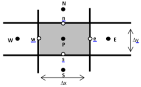
To approximate the gradient of $v_{0} \mathrm{~A}(\mathrm{t})$ in expressions of the cell-center values we use the 2D mesh given in Figure 2, where the cell-centers are appointed by uppercase letter (E,W,N,S) and the cell-faces are denoted by the lowercase ones (e,w,n,s).
Figure 2. Control volume mesh
After mathematical development of Eq. (15) we obtain Eq. (16) as fellows:
$\sum_{f} v_{0} \nabla A(t) \cdot \hat{n}_{f} s_{f}=v_{0}\left(\frac{A_{E}-A_{p}}{\Delta x}-\frac{A_{p}-A_{w}}{\Delta x}\right) \Delta y$
$+v_{0}\left(\frac{A_{N}-A_{p}}{\Delta x}-\frac{A_{p}-A_{S}}{\Delta x}\right) \Delta x$ (16)
The source term of Eq. (14) noted “F” can be expressed by:
$F=-j_{s}(t) \Delta y \times \Delta x-\left(\left(M_{y}\right)_{e}-\left(M_{y}\right)_{w}\right) \Delta y+$
$\left(\left(M_{x}\right)_{n}-\left(M_{x}\right)_{s}\right) \Delta x$ (17)
Finally, we can express all unknowns at the cell-centers of the mesh, which lead to obtain the matrix system of the following form:
$[a][A]_{t}=[D]\left[J_{s}\right]_{t}+\left[K^{x} K^{y}\right]\left[\begin{array}{l}M_{N, S}^{x} \\ M_{E, W}^{y}\end{array}\right]_{t-\Delta t}$ (18)
In Eq. (18), [A]t is the values at nodes of the potential vector, [JS]t represents the current source, [D] and [K] are the stiffness matrix, [M]t-Δt, is the magnetization term.
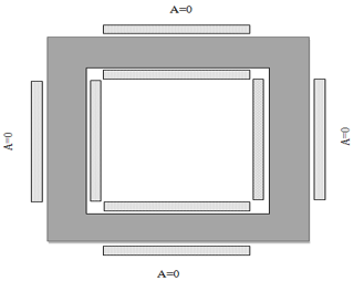
The FVM-DEM is applied to Epstein-frame constituting the bench of measure where the magnetic core is composed by FeSi 3% non-oriented grain magnetic material. The sheet is characterized by 0.35 mm thickness, 15 mm width, 147 mm length, and 7650 kg/m3 mass density; Figure 3, shows the Epstein framework.
Figure 3. Epstein framework
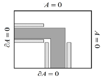
The symmetry of the system allows to study only a quarter (1/4) of the domain. Figure 4, shows a quarter (¼) of Epstein frame, with boundary conditions.
Figure 4. Epstein frame domain with boundary conditions
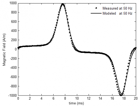
For the purpose of verifying the proposed method, a set of results is given in Figures 5-10, in which the average hysteresis loops and magnetic field waveform obtained by FVM-DEM are compared with the measured results for different frequencies. Figures 5 and 6, illustrate the magnetic field waveform and hysteresis loops of both measured and modeled at 50 Hz, let’s note that there is good agreement between the modeled and the experimental data. On the other hand, it demonstrated the accuracy of the identification method for determining dynamic parameters.
Figure 5. Magnetic field waveform modeled and measured at 50 Hz
Figure 6. Hysteresis loops modeled and measured at 50 Hz
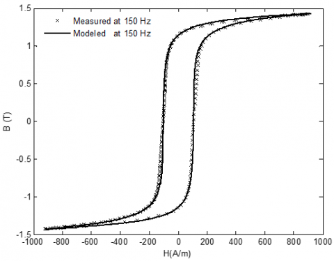
The obtained results are compared with measurements at distinct frequencies (150 Hz and 200 Hz). Figures 7-10 show a good agreement for both measured and modeled.
Figure 7. Hysteresis loops modeled and measured at 150 Hz
Figure 8. Magnetic field waveform modeled and measured at 150 Hz
Figure 9. Hysteresis loops modeled and measured at 200 Hz
Figure 10. Magnetic field waveform modeled and measured at 200 Hz
The combined of finite control volume method and the dynamic energetic model (FVM-DEM) were applied to solve dynamic hysteresis problem. A new formulation is proposed for modeling dynamic effects of magnetic field in ferromagnetic materials. This formulation allows to easily introducing the calculation of eddy current and anomalous losses.
To describe the dynamic behaviour in ferromagnetic materials, the energetic model is modified by introducing two additional energies associated with classical eddy and excess losses. Thus two new parameters related to eddy and excess losses are introduced. The dynamic energetic model is characterised by nine parameters seven of them are identified in quasi-static regime, and the two additional parameters are identified in dynamic regime. The new model is applicable in both quasi-static and dynamic cases.
The proposed methodology has good performances with regard to numerical and gives very satisfactory by comparison between measured and modelled hysteresis loops.
|
A |
Potential vector magnetic, T.m-1 |
|
B |
Magnetic induction, T |
|
Js |
Excitation current density, A.m-2 |
|
H M T |
Magnetic field, A.m-1 Magnetization, A.m-1 time, s |
|
Greek symbols |
|
|
ν0 |
Magnetic reluctivity of vacuum [H/m]-1 |
[1] Hamimid, M., Mimoune, S.M., Feliachi, M. (2013). Incorporation of modified dynamic inverse Jiles-Atherton model in finite volume time domain for nonlinear electromagnetic field computation. Journal of Applied Physics, 113(1): 013915. https://doi.org/10.1063/1.4773535
[2] Hamimid, M., Mimoune, S.M., Feliachi, M. (2011). Hybrid magnetic field formulation based on the losses separation method for modified dynamic inverse Jiles-Atherton model. Physica B: Condensed Matter, 406(14): 2755-2757. https://doi.org/10.1016/j.physb.2011.04.021
[3] Baghel, A.P.S., Kulkarni, S.V. (2014). Dynamic loss inclusion in the Jiles-Atherton (JA) hysteresis model using the original JA approach and the filed separation approach. IEEE Transactions on Magnetics, 50(2): 369-372. https://doi.org/10.1109/TMAG.2013.2284381
[4] Sadowski, N., Batistela, N.J., Bastos, J.P.A., Lajoie-Mazenc, M. (2002). An inverse Jiles-Atherton model to take into account hysteresis in time stepping finite-element calculations. IEEE Transactions on Magnetics, 38(2): 797-800. https://doi.org/10.1109/20.996206
[5] Kadota, Y., Morita, T. (2012). Preisach modeling of electric-field-induced strain of ferroelectric material considering 90° domain switching. Japanese Journal of Applied Physics, 51(951). https://doi.org/10.1143/JJAP.51.09LE08
[6] Bertotti, G. (1992). Dynamic generalization of the scalar preisach model of hysteresis. IEEE Transactions on Magnetics, 28(5): 2599-2601. https://doi.org/10.1109/20.179569
[7] Hauser, H. (1994). Energetic model of ferromagnetic hysteresis. Journal of Applied Physics, 75(5): 2584-2597. https://doi.org/10.1063/1.356233
[8] Hauser, H. (2004). Energetic model of ferromagnetic hysteresis: Isotropic magnetization. Journal of Applied Physics, 96(5): 2753-2767. https://doi.org/10.1063/1.1771479
[9] Mayergoyz, I.D. (1991). Mathematical Models of Hysteresis. Springer-Verlag New York. https://doi.org/10.1007/978-1-4612-3028-1
[10] Jiles, D.C., Atherton, D.L. (1986). Theory of ferromagnetic hysteresis. Journal of Magnetism and Magnetic Materials, 61(1-2): 48-60. https://doi.org/10.1016/0304-8853(86)90066-1
[11] Chiampi, M., Chiarabaglio, D., Repetto, M. (1995). A Jiles–Atherton and fixed-point combined technique for time periodic magnetic field problems with hysteresis. IEEE Transactions on Magnetics, 31(6): 4306-4311. https://doi.org/10.1109/20.488295
[12] Muramatsu, K., Takahashi, N., Nakata, T., Nakano, M., Ejiri, Y., Takehara, J. (1997). 3-D time-periodic finite element analysis of magnetic field in nonoriented materials taking into account hysteresis characteristics. IEEE Transactions on Magnetics, 33(2): 1584-1587. https://doi.org/10.1109/20.582569
[13] Ionel, D.M., Popescu, M., Dellinger, S.J., Miller, T.J.E., Heideman, R.J., McGilp, M.I. (2006) On the variation with flux and frequency of the core loss coefficients in electrical machines. IEEE Transactions on Magnetics, 42(3): 658-667. https://doi.org/10.1109/TIA.2006.872941
[14] Ionel, D.M., Popescu, M., McGilp, M.I., Miller, T.J.E., Dellinger, S.J., Heideman, R.J. (2007). Computation of core losses in electrical machines using improved models for laminated steel. IEEE Transactions on Magnetics, 42(6): 1554-1564. https://doi.org/10.1109/TIA.2007.908159
[15] Bertotti, G. (1988). General properties of power losses in soft ferromagnetic materials. IEEE Transactions on Magnetics, 24(1): 621-630. https://doi.org/10.1109/20.43994
[16] Bertotti, G. (1991). Generalized preisach model for the description of hysteresis and eddy current effects in metallic ferromagnetic materials. Journal of Applied Physics, 69(8): 4608-4610. https://doi.org/10.1063/1.348325 [17] Zirka, S.E., Moroz, Y.I., Marketos, P., Moses, A.J. (2004). Dynamic hysteresis modelling. Physica B: Condensed Matter, 343(1-4): 90-95. https://doi.org/10.1016/j.physb.2003.08.036
[18] Hamimid, M., Mimoune, S.M., Feliachi, M. (2011). Dynamic formulation for energetic model compared with hybrid magnetic formulation of ferromagnetic hysteresis. International Journal of Numerical Modelling, 30(6):1-5. https://doi.org/10.1002/jnm.2225
[19] Chandrasena, W., McLaren, P.G., Annakkage, U.D., Jayasinghe, R.P., Muthumuni, D., Dirks, E. (2006). Simulation of hysteresis and eddy current effects in a power transformer. Electric Power Systems Research, 76(8): 634-641. https://doi.org/10.1016/j.epsr.2005.12.009
[20] Jiles, D.C. (1994). Modelling the effects of eddy current losses on frequency dependent hysteresis in electrically conducting media. IEEE Transactions on Magnetics, 30(6): 4326-4328. https://doi.org/10.1109/20.334076
[21] Hamimid, M., Mimoune, S.M., Feliachi, M. (2012). Minor hysteresis loops model based on exponential parameters scaling of the modified Jiles–Atherton model. Physica B: Condensed Matter, 407(13): 2438-2441. https://doi.org/10.1016/j.physb.2012.03.042