Mohammed Elmahfoud* | Badre Bossoufi | Mohammed Taoussi | Najib El Ouanjli | Aziz Derouich
© 2020 IIETA. This article is published by IIETA and is licensed under the CC BY 4.0 license (http://creativecommons.org/licenses/by/4.0/).
OPEN ACCESS
In this paper, a comparative study between field oriented control and Backstepping adaptive control for a doubly fed induction motor (DFIM) is proposed. At the beginning, the mathematical model of the DFIM is presented. Thereafter, these control strategies are described and designed, then implemented using the Matlab/Simulink environment. Finally, the different strategies are compared in terms of static and dynamic error, response time, overshoot and robustness. The results of the comparison clearly show that the Backstepping adaptive control provides better performance and is characterized by high robustness vis-a-vis parametric variations.
control motor, DFIM, adaptive, Lyapunov
The doubly fed induction machine (DFIM) is widely used in the domain of the conversion of mechanical energy to electrical energy such as: wind and hydraulic systems [1, 2], and also in motor mode operation like: marine propulsion, metallurgy (rolling), rail traction, pumping and electric/hybrid vehicles [3].
The DFIM is characterized by low cost, efficiency and simplicity of manufacture. An increasing interest is being given to this machine [4]. This interest is due to:
• A greater number of freedom degrees related to the accessibility of rotor variables.
• A greater operating flexibility due to the presence of static converters associated with the two armatures.
• A widening of the speed range for operation at constant flux and maximum torque.
However, the DFIM is a non-linear machine due to the coupling between the flux and electromagnetic torque, which requires a control strategy that allows these variables to be decoupled.
For this reason, several techniques have been developed to control the DFIM with variable speed and to obtain a decoupling between the control variables. The vector control strategy by flux orientation (FOC) was introduced by Blaschke and Hasse [5, 6]. The purpose of this technique is to control the induction machine as a direct current machine with independent excitation, where there is a natural decoupling between the magnitude controlling torque and flux [7]. The application of the latter to the doubly-fed induction machine offers an attractive solution for obtaining better performance in terms of rapidity, precision and stability. But, the conception of this control is based on the use of classical proportional-integral (PI) regulators which are not very efficient when the system is disturbed, hence the sensitivity of FOC to parametric variations [8, 9].
To overcome these inconveniences, various strategies have been proposed to replace PI controllers and improve the performance and robustness of systems based on the DFIM. The Backstopping technique is a recursive method (step by step). At each step, a virtual control is calculated to ensure the convergence of the system towards its equilibrium state. This can be obtained by using the Lyapunov functions which ensure step by step the stabilization of each synthesis step. However, all these control techniques are based on the knowledge of the parameters of the system to be controlled. In the presence of parameter uncertainties, there is no guarantee that the operation will meet the specifications. In this case, it is preferable to use an adaptive control to estimate these parameters. The adaptive Backstepping is the method that results from the fusion of adaptive design and the recursive technique of non-adaptive Backstepping. However, the direct combination of these two methods leads to finding a triplet (Lyapunov function, control law, adaptation law). The construction of this triplet is done simultaneously. The three operations are intertwined, allowing for the different destructive effects to be taken into account, in order to preserve the stability of the system. The growing interest in this approach is mainly due to its wide applicability to industrial processes, but the problem of its analytical formulation is also raised [10, 11].
The aim of this work is to make a comparative study between two controls: the FOC control and the Backstepping control. It is worth noting that several studies have been devoted in recent decades to investigating and improving Backstepping and FOC controls, but few publications are close to comparing the advantages and disadvantages.
This document is organized as follows: Section 2 is interested in the modeling of the machine studied in reference frame (d,q). Section 3 presents the principle and results of the FOC control applied to DFIM. The adaptive Backstepping control of the DFIM is designed in section 4. The comparative study between the two techniques studied is summarized in the Table 2 in section 5. Finally, section 6 displays the conclusions of the document and recommendations for future work.
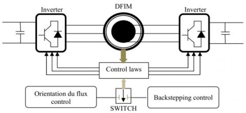
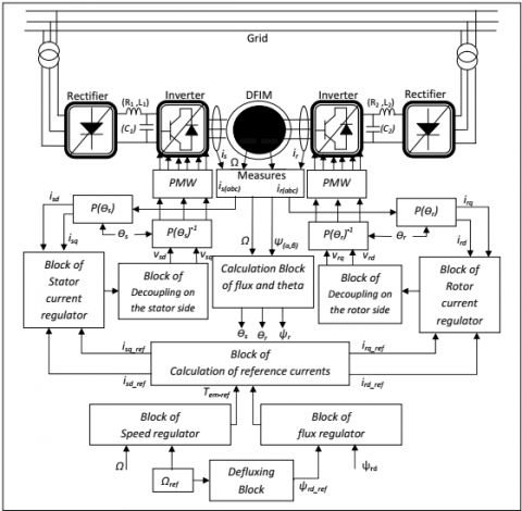
The doubly fed induction motor is powered by two voltage inverters which are connected to two DC bus voltages. Figure 1 illustrates the block diagram of the system studied [12].
Figure 1. General diagram of the studied system
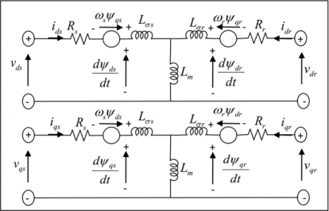
The DFIM equivalent circuit in the reference (d,q) is shown in Figure 2.
Figure 2. Electrical diagram of the DFIM
After the Park transformation, the DFIM model is defined by the equations [13, 14]:
$\left\{\begin{array}{l}
v_{s d}=R_{s} \cdot i_{s d}+\frac{d}{d t} \psi_{s d}-\frac{d \theta_{s}}{d t} \cdot \psi_{s q} \\
v_{s q}=R_{s} \cdot i_{s q}+\frac{d}{d t} \psi_{s q}+\frac{d \theta_{s}}{d t} \cdot \psi_{s d} \\
v_{r d}=R_{r \cdot} i_{r d}+\frac{d}{d t} \psi_{r d}-\frac{d \theta_{r}}{d t} \cdot \psi_{r q} \\
v_{r q}=R_{r \cdot} i_{r q}+\frac{d}{d t} \psi_{r q}+\frac{d \theta_{r}}{d t} \cdot \psi_{r d}
\end{array}\right.$ (1)
$\left\{\begin{aligned}
i_{s d} &=\frac{1}{\sigma L_{s}} \psi_{s d}-\frac{M}{\sigma L_{s} L_{r}} \cdot \psi_{r d} \\
i_{s q} &=\frac{1}{\sigma L_{s}} \psi_{s q}-\frac{M}{\sigma L_{s} L_{r}} \cdot \psi_{r q} \\
i_{r d} &=-\frac{M}{\sigma L_{s} L_{r}} \psi_{s d}+\frac{1}{\sigma L_{r}} \cdot \psi_{r d} \\
i_{r q} &=-\frac{M}{\sigma L_{s} L_{r}} \psi_{s q}+\frac{1}{\sigma L_{r}} \cdot \psi_{r q}
\end{aligned}\right.$ (2)
with: $\sigma=1-\frac{M}{L_{s} L_{r}} \text { et } M=M_{s r}=M_{r s}$ .
$\left\{\begin{array}{l}
\psi_{s d}=L_{s} \cdot i_{s d}+M \cdot i_{r d} \\
\psi_{s q}=L_{s} \cdot i_{s q}+M \cdot i_{r q} \\
\psi_{r d}=L_{r} \cdot i_{r d}+M \cdot i_{s d} \\
\psi_{r q}=L_{r} \cdot i_{r q}+M \cdot i_{s q}
\end{array}\right.$ (3)
$\left\{\begin{array}{c}
T_{e m}=T_{r}+J \frac{d \Omega}{d t}+f . \Omega \\
T_{e m}=p \cdot\left(\psi_{s q} \cdot \mathrm{i}_{s d}-\psi_{s d} \cdot \mathrm{i}_{s q}\right)
\end{array}\right.$ (4)
The objective of this control is to obtain a simple model of the DFIM that makes it similar to that of a direct current machine with separate excitation. The fundamental idea is to transform the electrical variables into a reference frame that rotates with the flux vector. It consists in orienting the flux vector along one of the axes of the Park reference frame, so that the flux is controlled by the direct current component and the torque is controlled by the other component [15, 16].
3.1 Application of the FOC to DFIM
The application of this control to DFIM consists in decoupling the variables that generate torque and flux. The rotor field oriented control is based on aligning the rotor flux along the d-axis of the rotating reference frame. As a result, we obtain: $\psi_{r d}=\psi_{r} \text { and } \psi_{r q}=0$ .
From the Eq. (3):
$\psi_{r q}=0 \Leftrightarrow\left\{\begin{array}{l}
i_{r q}=-\frac{M}{L_{r}} \cdot i_{s q} \\
i_{s q}=-\frac{L_{r}}{M} \cdot i_{r q}
\end{array}\right.$ (5)
The electromagnetic torque is expressed as:
$T_{e m}=p \cdot\left(\psi_{r q} \cdot i_{r d}-\psi_{r d} \cdot i_{r q}\right)=-p \cdot \psi_{r d} \cdot i_{r q}$ (6)
By applying a unit power factor to the rotor:
$i_{r q}=0 \Leftrightarrow i_{s d}=\frac{\psi_{r d}}{M}$ (7)
To achieve a successful decoupling between the d and q axes, the intermediate voltages are defined by the below equations:
$\left\{\begin{array}{l}
V_{t s d}=V_{s d}+\frac{M}{L_{r}} \cdot V_{r d} \\
V_{t s q}=V_{s q}+\frac{M}{L_{r}} \cdot V_{r q} \\
V_{t r d}=V_{r d}+\frac{M}{L_{s}} \cdot V_{s d} \\
V_{t r q}=V_{r q}+\frac{M}{L_{s}} \cdot V_{s q}
\end{array}\right.$ (8)
We obtain the following from Eqns. (1), (3) and (8):
$\left\{\begin{array}{c}
V_{t s d}=R_{s} \cdot i_{s d}+\sigma \cdot L_{s} \frac{d \mathrm{i}_{s d}}{d t}-R_{r} \frac{M}{L_{r}} \cdot \mathrm{i}_{r d}-\psi_{s q} \omega_{s} \\
+\frac{M}{L_{r}} \psi_{r q}\left(\omega_{s}-\omega\right) \\
V_{t s q}=R_{s} \cdot t_{s q}+\sigma \cdot L_{s} \frac{d i_{s q}}{d t}-R_{r} \frac{M}{L_{r}} \cdot \mathrm{i}_{r q}-\psi_{s d} \omega_{s} \\
+\frac{M}{L_{r}} \psi_{r d}\left(\omega_{s}-\omega\right) \\
V_{t r d}=R_{r \cdot \cdot} i_{r d}+\sigma \cdot L_{r} \frac{d \mathrm{i}_{r d}}{d t}-R_{s} \frac{M}{L_{s}} \cdot \mathrm{i}_{s d}-\psi_{r q}\left(\omega_{s}-\omega\right) \\
+\frac{M}{L_{r}} \psi_{s q} \omega_{s} \\
V_{t r q}=R_{r} \cdot i_{r q}+\sigma \cdot L_{r} \frac{d \mathrm{i}_{r q}}{d t}-R_{e} \frac{M}{L_{s}} \cdot \mathrm{i}_{s q}-\psi_{r d}\left(\omega_{s}-\omega\right) \\
+\frac{M}{L_{r}} \psi_{s d} \omega_{s}
\end{array}\right.$ (9)
With:
$\left\{\begin{aligned}
V_{t s d}=V_{t s d c}+V_{t s d c 1} &=R_{s} \cdot i_{s d}+\sigma \cdot L_{s} \frac{d \mathbf{i}_{s d}}{d t}+V_{t s d c 1} \\
V_{t s q}=V_{t s q c}+V_{t s q c 1} &=R_{s} \cdot i_{s q}+\sigma \cdot L_{s} \frac{d i_{s q}}{d t}+V_{t s q c 1} \\
V_{t r d}=V_{t r d c}+V_{t r d c 1} &=R_{r \cdot t} i_{r d}+\sigma \cdot L_{r} \frac{d i_{r d}}{d t}+V_{t r d c 1} \\
V_{t r q}=V_{t r a c}+V_{t r q c 1} &=R_{r \cdot t} i_{r q}+\sigma \cdot L_{r} \frac{d i_{r q}}{d t}+V_{t r q c 1}
\end{aligned}\right.$
$V_{\text {tsdc } 1} \quad, \quad V_{\text {tsqc } 1} \quad, \quad V_{\text {tqdc } 1}$ and $\quad V_{\text {trqc } 1}$ are regarded as compensation conditions.
The functions of transfer connecting the rotor and stator components of each axis are:
$\left\{\begin{array}{l}
\frac{I_{s d}}{V_{t s d c 1}}=\frac{I_{s d}}{V_{t s d c 1}}=\frac{1}{R_{s+} \sigma \cdot L_{s} \cdot s} \\
\frac{I_{r d}}{V_{t r d c 1}}=\frac{I_{r d}}{V_{t r d c 1}}=\frac{1}{R_{r+} \sigma \cdot L_{r} \cdot s}
\end{array}\right.$ (10)
From the expressions of the established equations, a summary connection table can be drawn up setting the aims of the control strategy with the references of the action variables involved (Table 1):
Table 1. Reference currents
|
Objective |
Reference currents |
|
$\psi_{\mathrm{rd}}=\psi_{\mathrm{r}}$ |
$\mathrm{I}_{\mathrm{sd}}^{*}=\frac{1}{\mathrm{M}} \psi_{\mathrm{rd}}^{*}$ |
|
$\psi_{\mathrm{rq}}=0$ |
$\mathrm{I}_{\mathrm{sq}}^{*}=\frac{\mathrm{L}_{\mathrm{r}}}{\mathrm{p} . \mathrm{M} \cdot \psi_{\mathrm{rd}}^{*}} \mathrm{T}_{\mathrm{em}}^{*}$ |
|
Qr=0, (cos φ=1) |
$I_{r d} *=0$ |
|
$\mathrm{T}_{\mathrm{em}}^{*}=\mathrm{T}_{\mathrm{em}}$ |
$\mathrm{I}_{\mathrm{rq}}^{*}=-\frac{1}{\mathrm{p} \cdot \psi_{\mathrm{rd}}^{*}} \mathrm{T}_{\mathrm{em}}^{*}$ |
Figure 3. Synoptic schema of the FOC applied to DFIM
Figure 3 above shows the FOC principle applied to the DFIM.
3.2 Simulation result
In order to test the performance and robustness of the system, several series of numerical simulations were implemented for the DFIM in the Matlab/Simulink environment. The motor parameters used are presented in appendix B.
3.2.1 Performance tests
In this section, two performance tests are performed:
(a) Rotation speed
(b) Electromagnetic torque
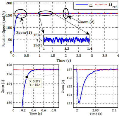
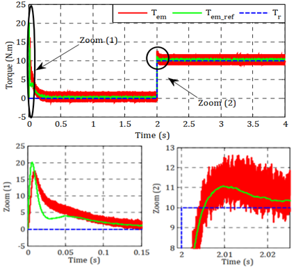
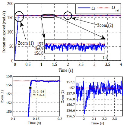
Figure 4. Simulation results with speed step
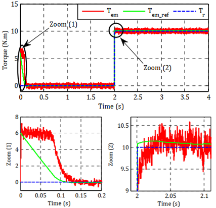
Figure 4 shows the simulation of FOC for a speed step with introduction of a load $T_{r}=10 N . m$. Figure (4.a) illustrates that rotation speed follows the reference value with a response time of 271ms and static error of about ±0.3rad/s. Moreover, when a perturbation is applied, a relative drop of 3.93rad/s appears, the rejection time equal to 60ms. Figure (4.b) presents that the torque practically returns to zero at the end of the transitory mode and the starting torque is equal to 20N.m. We also observe that when applying the load torque at t=2s the electromagnetic torque follows its reference value with a band of $\Delta T_{e m}=\pm 3.5 \mathrm{N} . \mathrm{m}$, because the controller reacts instantly to the reference electromagnetic torque.
(a) Rotation speed
(b) Speed error
(c) Electromagnetic torque
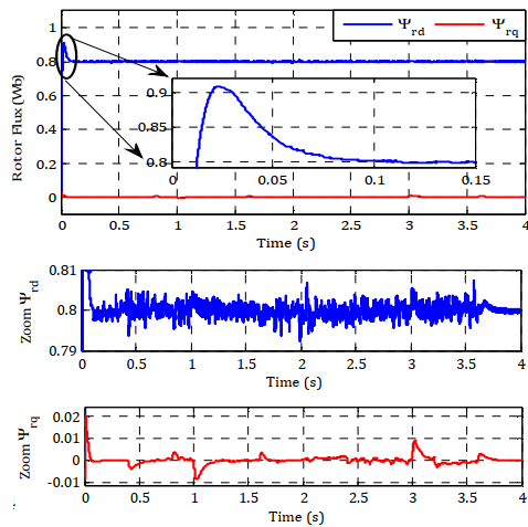
(d) Rotor flux
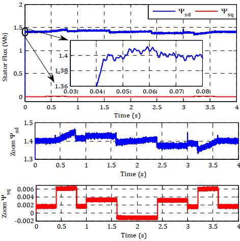
(e) Stator flux
(f) Rotor currents
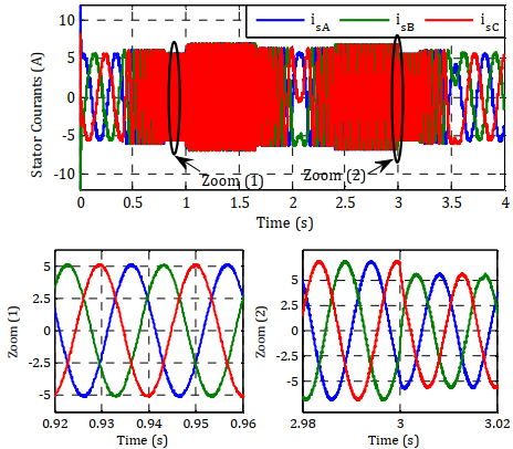
(g) Stator currents
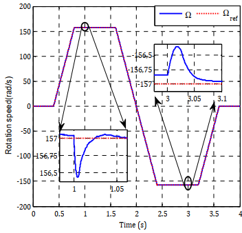
Figure 5. Simulation results with trapezoidal speed
Figure 5 illustrates the simulation results of the FOC applied to the DFIM tested by a trapezoidal speed set-point with the application of load torque $T_{r}=10 N . m$ at t=1s. These results show that:
The stator and rotor currents shown in Figures (5.f and 5.g) are sinusoidal and present variations in amplitude proportional to changes in torque and direction of rotation.
3.2.2 Robustness tests
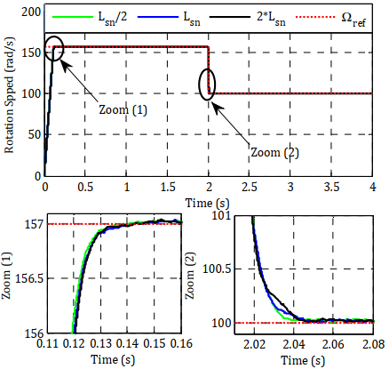
In the aim of testing the robustness of FOC, we will study the influence of parametric variations (inductances and resistances) on this control. Figure.6 represents the dynamic behavior of the speed in this test.
From the results presented in Figure 6, we observe that the excessive parametric variation performed on DFIM produced clear effects on the speed curves. However, a variation in the resistance or inductance from its nominal value affects the response time, rise time and static error.
(a) Rotor resistance
(b) Stator resistance
(c) Rotor inductance
(d) Stator inductance
Figure 6. Robustness tests for a variation
The influence of rotor resistance comes from the important role it plays in decoupling. One of its advantages is its independence from the variation of stator resistance, the fact that the latter has no role in the design of the control, in particular from the point of view of decoupling.
The variation of the rotor inductance does not have a remarkable influence on the speed, but on the orientation of the flux. On the other hand, the effect of the variation in stator inductance is not negligible, that is to say, the control partially loses the control efficiency but still maintains the decoupling between torque and flux.
The majority of non-linear controls are based on the Lyapunov stability theory. The purpose is to find a control law that makes the derivative of a Lyapunov function, chosen a priori, defined or semi defined negative [17, 18]. The principal difficulty is in the right choice of a suitable Lyapunov function. The Backstepping technique overcomes this difficulty by gradually building a Lyapunov function adapted to the system and allows deducing the control that makes the derivative of this function negative. This ensures that, at all times, the global asymptotic stability of non-linear systems in tracking and regulation [19, 20].
The application of the Backstepping control is done according to the system parameters. If the parameters are known, we used the non-adaptive Backstepping control, else we need an adaptation law, we say that the control used is the adaptive Backstepping control. The adaptive version of Backstepping offers an iterative and systematic method, which allows for non-linear systems of all orders.
4.1 Application of adaptive Backstepping control to the DFIM
The principle objective of non-linear adaptive Backstepping control applied to the DFIM is to allow speed control according to its reference value ($\Omega_{\text {ref }}$) without taking into account external disturbances and internal variations. We propose to remove the classical PI regulators in the scheme of the FOC given in Figure 3 and replace them with adaptive Backstepping control laws. According to electrical, magnetic and mechanical equations of the DFIM, the instant expressions can be written as follows:
$\left\{\begin{array}{l}
\frac{d \psi_{r d}}{d t}=v_{r d}+\frac{R_{r \cdot} M}{\sigma \cdot L_{r \cdot L_{s}}} \psi_{s d}-\frac{R_{r}}{\sigma \cdot L_{r}} \psi_{r d}+\psi_{r q} \omega_{r} \\
\frac{d \psi_{r q}}{d t}=v_{r q}+\frac{R_{r \cdot} M}{\sigma \cdot L_{r \cdot} L_{s}} \psi_{s q}-\frac{R_{r}}{\sigma \cdot L_{r}} \psi_{r q}+\psi_{r d} \omega_{r}
\end{array}\right.$ (11)
$\left\{\begin{array}{l}
\frac{d \psi_{s d}}{d t}=v_{s d}+\frac{R_{s} \cdot M}{\sigma \cdot L_{r} \cdot L_{s}} \psi_{r d}-\frac{R_{s}}{\sigma \cdot L_{s}} \psi_{s d}+\psi_{s q} \omega_{s} \\
\frac{d \psi_{s q}}{d t}=v_{s q}+\frac{R_{s} \cdot M}{\sigma \cdot L_{r} \cdot L_{s}} \psi_{r q}-\frac{R_{s}}{\sigma \cdot L_{s}} \psi_{s q}+\psi_{s d} \omega_{s}
\end{array}\right.$ (12)
$\begin{array}{c}
\frac{d \Omega}{d t}=\frac{p \cdot(1-\sigma)}{J \cdot \sigma \cdot M}\left(\psi_{r d} \psi_{s q}-\psi_{r q} \psi_{s d}\right)+ \\
\frac{T_{r}}{J}+\frac{f}{J} \Omega
\end{array}$ (13)
With:
$[X]=\left[\psi_{r d} \psi_{r q} \psi_{s d} \psi_{s q} \Omega\right]^{T}$: Status vector (measurable or estimated).
$[U]=\left[\begin{array}{llll}
v_{r d} & v_{r q} & v_{s d} & v_{s q}
\end{array}\right]^{T}$: Variable of control.
It is evident that the dynamic model of speed is very highly non-linear because of the coupling between velocity and magnetic flux (13). To do this, the study of the stability of the system then consists in searching for a Lyapunov function V(x) of defined sign. Since the DFIM equations are of second order, the implementation is carried out in three steps, one for speed control, the other for magnetic flux control and the last one for estimating system parameters.
The objective of this step is to define the tracking error of the state variable ($e_{\Omega}$) which represents the error between the actual speed Ω (measured or estimated) and the reference speed $\Omega_{r e f}$ , So:
$e_{\Omega}=\Omega_{r e f}-\Omega$ (14)
The combination of the Backstepping method with FOC gives the DFIM control interesting robustness qualities, and further strengthens the Backstepping robustness. Therefore, Eq. (14) becomes as follows:
$\begin{array}{c}
e_{\Omega}=\Omega_{r e f}-\Omega \\
=\Omega_{r e f}-\frac{p \cdot(1-\sigma)}{J \cdot \sigma \cdot M}\left(\psi_{r d} \psi_{s q}\right)+\frac{T_{r}}{J}+\frac{f}{J}
\end{array}$ (15)
To take into account this Eq. (15), the Lyapunov function is defined as follows:
$V_{1}=\frac{1}{2} e_{\Omega}^{2}$ (16)
In order to ensure the system stability, the derivative of the Lyapunov function V1 must be made negative. To do this, we defined a positive constant (kΩ) to the derivative of the Eq. (16). After development:
$\begin{array}{l}
\dot{V}_{1} \\
=-K_{\Omega} e_{\Omega}^{2}
\end{array}$$+e_{\Omega \cdot}\left[\begin{array}{c}
K_{\Omega \cdot} e_{\Omega}+\dot{\Omega}_{r e f} \\
-\frac{p \cdot(1-\sigma)}{J \cdot \sigma \cdot M}\left(\psi_{r d} \psi_{s q}\right)+\frac{T_{r}}{J}+\frac{f}{J} \Omega
\end{array}\right]$ (17)
According to this Eq. (17) and the stability condition of Lyapunov function, we consider magnetic flux as the virtual inputs of the DFIM. So:
$\left\{\begin{array}{c}
\psi_{\text {sqref}}=\frac{1}{\frac{p \cdot(1-\sigma)}{J \cdot \sigma \cdot M} \psi_{\text {rdref}}}\left(K_{\Omega \cdot} e_{\Omega}+\frac{T_{r}}{J}+\frac{f}{J} \Omega\right) \\
\psi_{\text {sdref}}=\psi_{s} \\
\psi_{r d_{\text {ref}}}=\psi_{r} \\
\psi_{r q_{\text {ref}}}=0
\end{array}\right.$ (18)
The Eq. (18) is replaced in Eq. (17) and the speed reference $\Omega_{\text {ref }}$ is assumed to be constant. The negativity of the derivative of V1 is then expressed as follows:
$\dot{V}_{1}=-K_{\Omega} \cdot e_{\Omega}^{2} \leq 0$ (19)
This solution is designed to stabilize the first step. The state of the magnetic flux is chosen as the virtual control of the speed state, then a virtual control of the flux is defined, which will be processed in the second step.
In this step, the errors between the real flux components (measured or estimated) and reference flux are defined, such as:
$\left\{\begin{array}{l}
e_{\psi_{r d}}=\psi_{r d_{-} r e f}-\psi_{r d} \\
e_{\psi_{r d}}=\psi_{r d_{r e f}}-\psi_{r d} \\
e_{\psi_{s d}}=\psi_{s d_{-} r e f}-\psi_{s d} \\
e_{\psi_{s d}}=\psi_{s d_{-} r e f}-\psi_{s d}
\end{array}\right.$ (20)
From the Eq. (20), the real control laws
($v_{s d}, v_{s q}, v_{r d} \text { and } v_{r q}$) of DFIM will be designed. In order to extract these control laws, another term V2 added to the previous Lyapunov function V1, such as:
$V_{2}=\frac{1}{2}\left(e_{\Omega}^{2}+e_{\psi_{\mathrm{rd}}}^{2}+e_{\psi_{\mathrm{rq}}}^{2}+e_{\psi_{\mathrm{sd}}}^{2}+e_{\psi_{\mathrm{sq}}}^{2}\right)$ (21)
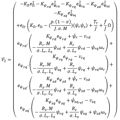
To guarantee the stability of the system, it is necessary to ensure the negativity of the derivative of the V2. To do this, the positive constants ($\mathrm{k}_{\psi}>0$) are defined for the derivative of the Eq. (21). After the development:
(22)
From the Eq. (22) and the stability condition of Lyapunov function, the control laws ($v_{s d}, v_{s q}, v_{r d} \text { and } v_{r q}$) applied to the DFIM in engine mode are obtained, such as:
$\left\{\begin{array}{c}
v_{r d}=K_{\psi_{r d}} e_{\psi_{r d}}+\dot{\psi}_{r}-\frac{R_{r} \cdot M}{\sigma \cdot L_{r \cdot} L_{s}} \psi_{s d}+\frac{R_{r}}{\sigma \cdot L_{r}} \psi_{r d}-\psi_{r q} \omega_{r} \\
v_{r q}=K_{\psi_{r q}} e_{\psi_{r q}}-\frac{R_{r \cdot} M}{\sigma \cdot L_{r} \cdot L_{s}} \psi_{s q}+\frac{R_{r}}{\sigma \cdot L_{r}} \psi_{r q}+\psi_{r d} \omega_{r} \\
v_{s d}=K_{\psi_{s d}} e_{\psi_{s d}}+\dot{\psi}_{s}-\frac{R_{s} \cdot M}{\sigma \cdot L_{r \cdot L_{s}}} \psi_{r d}+\frac{R_{s}}{\sigma \cdot L_{s}} \psi_{s d}-\psi_{s q} \omega_{s} \\
v_{s q}=K_{\psi_{s q}} e_{\psi_{s q}}+\dot{\psi}_{s q_{r e f}}-\frac{R_{s} \cdot M}{\sigma \cdot L_{r \cdot} L_{s}} \psi_{r q}+\frac{R_{s}}{\sigma \cdot L_{s}} \psi_{s q}+\psi_{s d} \omega_{s}
\end{array}\right.$ (23)
The Eq. (23) is replaced in Eq. (22), which implies the negativity of the derivative of V2, such that:
$\begin{array}{c}
\dot{V}_{2}=\left(\begin{array}{c}
-K_{\Omega} \cdot e_{\Omega}-K_{\psi_{r d}} e_{\psi_{r d}}-K_{\psi_{r q}} e_{\psi_{r q}} \\
-K_{\psi_{s d}} e_{\psi_{s d}}-K_{\psi_{s q}} e_{\psi_{s q}}
\end{array}\right) \\
\leq 0
\end{array}$ (24)
The Eq. (24) implies asymptotic stability towards the origin and the output of the DFIM then follows its reference value.
In the above equations, the control laws are developed under the hypothesis that the DFIM parameters are invariant. This hypothesis is not always true. In fact, one of the problems encountered in controlling the DFIM concerns the variation of its internal parameters and external disturbances due to changes in temperature, the level of magnetic saturation in the machine and the variation in the load torque. The use of estimators improves the robustness of the machine against parametric variations and measurement noise.
To design the non-linear adaptive Backstepping control, the real parameters vector of the DFIM is replaced by its estimate. In this case, the control laws given by Eq. (23) will be reinforced by terms that will compensate for the transitions of the estimated parameters.
We have:
$\left\{\begin{array}{c}
\dot{e}_{\Omega}=\hat{a}_{1}\left(\psi_{r} \psi_{s}\right)+\frac{T_{r}}{J}+\frac{f}{J} \Omega \\
\dot{e}_{\psi_{r d}}=\dot{\psi}_{r}-v_{r d}-\hat{a}_{2} \psi_{s d}+\hat{a}_{3} \psi_{r d}-\psi_{r q} \omega_{r} \\
\dot{e}_{\psi_{r q}}=-v_{r q}-\hat{a}_{2} \psi_{s q}+\hat{a}_{3} \psi_{r q}+\psi_{r d} \omega_{r} \\
\dot{e}_{\psi_{s d}}=-v_{s d}+\dot{\psi}_{s}-\hat{a}_{4} \psi_{r d}+\hat{a}_{5} \psi_{s d}-\psi_{s q} \omega_{s} \\
\dot{e}_{\psi_{s q}}=-v_{s q}+\dot{\psi}_{s q_{r e f}}-\hat{a}_{4} \psi_{r q}+\hat{a}_{5} \psi_{s q}+\psi_{s d} \omega_{s}
\end{array}\right.$ (25)
With:
$\begin{aligned}
\hat{a}_{1}=\frac{p \cdot(1-\hat{\sigma})}{J \cdot \hat{\sigma} \cdot M} & ; \hat{a}_{2}=\frac{\hat{R}_{r} \cdot M}{\hat{\sigma} \cdot \hat{L}_{r} \cdot \hat{L}_{s}} ; \hat{a}_{3}=\frac{\hat{R}_{r}}{\hat{\sigma} \cdot \hat{L}_{r}} ; \\
\hat{a}_{4} &=\frac{\hat{R}_{s} \cdot M}{\hat{\sigma} \cdot \hat{L}_{r} \cdot \hat{L}_{s}} ; \hat{a}_{5}=\frac{\widehat{R}_{s}}{\hat{\sigma} \cdot \hat{L}_{s}}
\end{aligned}$
From the Eq. (26), a new function of Lyapunov V2 is defined, such as:
$\begin{array}{l}V_{2}=\frac{1}{2}\left(e_{\Omega}^{2}+e_{\psi_{\mathrm{rd}}}^{2}+e_{\psi_{\mathrm{rq}}}^{2}+e_{\psi_{\mathrm{sd}}}^{2}+e_{\psi_{\mathrm{sq}}}^{2}+\frac{\tilde{T}_{r}^{2}}{\gamma_{r}}+\frac{\tilde{a}_{1}^{2}}{\gamma_{1}}+\frac{\tilde{a}_{2}^{2}}{\gamma_{2}}+\right. \\\left.\frac{\tilde{a}_{3}^{2}}{\gamma_{3}}+\frac{\tilde{a}_{4}^{2}}{\gamma_{4}}+\frac{\tilde{a}_{5}^{2}}{\gamma_{5}}\right)
\end{array}$ (26)
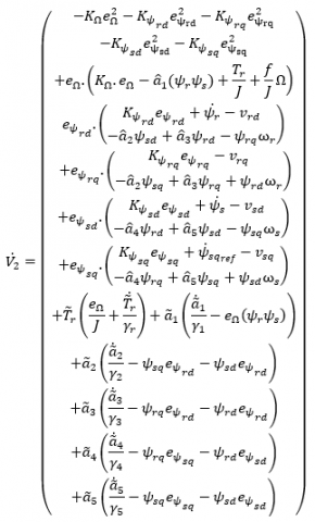
To ensure the system stability, the negativity of the derivative of the Eq. (27) must be guaranteed. To do this, the positive constants ($\mathrm{k}_{\psi}$)>0 is added to the derivative of this equation. The following expression is obtained after the calculation:
(27)
From Eq. (7), the control laws ($v_{s d}, v_{s q}, v_{r d} \text { and } v_{r q}$) applied to DFIM are obtained, such as:
$\left\{\begin{array}{c}
v_{r d}=K_{\psi_{r d}} e_{\psi_{r d}}+\dot{\psi}_{r}-\tilde{a}_{2}+\tilde{a}_{3} \psi_{r d}-\psi_{r q} \omega_{r} \\
v_{r q}=K_{\psi_{r q}} e_{\psi_{r q}}-\tilde{a}_{2} \psi_{s q}+\tilde{a}_{3} \psi_{r q}+\psi_{r d} \omega_{r} \\
v_{s d}=K_{\psi_{s d}} e_{\psi_{s d}}+\dot{\psi}_{s}-\tilde{a}_{4} \psi_{r d}+\tilde{a}_{5} \psi_{s d}-\psi_{s q} \omega_{s} \\
v_{s q}=K_{\psi_{s q}} e_{\psi_{s q}}+\dot{\psi}_{s q_{r e f}}-\tilde{a}_{4} \psi_{r q}+\tilde{a}_{5} \psi_{s q}+\psi_{s d} \omega_{s}
\end{array}\right.$ (28)
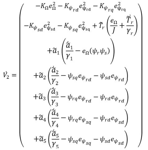
The Eq. (29) is replaced in Eq. (28), which simplifies the dynamics of the V2 derivative as follows:
(29)
From the Eq. (29), the adaptation expressions of the internal and external parameters of DFIM are obtained as follows:
$\tilde{T}_{r}=\int \dot{\tilde{T}}_{r}=\int-\frac{e_{\Omega}}{J} \cdot \gamma_{r}$ (30)
$\left\{\begin{array}{c}
\tilde{R}_{r}=\int \dot{\tilde{R}}_{r}=\int \dot{\tilde{\sigma}} \cdot \dot{\tilde{L}}_{r} \cdot \dot{\tilde{a}}_{3} \\
=\int-\dot{\tilde{\sigma}} \cdot \dot{\tilde{L}}_{r \cdot} \cdot \gamma_{3}\left(\psi_{r q} e_{\psi_{r q}}+\psi_{r d} e_{\psi_{r d}}\right) \\
\tilde{R}_{s}=\int \dot{\tilde{R}}_{s}=\int \tilde{\sigma} \cdot \dot{\tilde{L}}_{s} \cdot \dot{\tilde{a}}_{5} \\
=\int-\dot{\tilde{\sigma}} \cdot \dot{\tilde{L}}_{s} \cdot \gamma_{5}\left(\psi_{z q} e_{\psi_{z q}}+\psi_{s d} e_{\psi_{s d}}\right)
\end{array}\right.$ (31)
$\left\{\begin{array}{l}
\tilde{L}_{r}=\int \dot{\tilde{L}}_{r}=\int M \cdot \frac{\dot{\tilde{a}}_{5}}{\dot{\tilde{a}}_{4}}=\int-\frac{\gamma_{5}\left(\psi_{s d} e_{\psi_{s d}}+\psi_{s q} e_{\psi_{s q}}\right)}{\gamma_{4}\left(\psi_{r q} e_{\psi_{s q}}+\psi_{r d} e_{\psi_{s d}}\right)} \\
\tilde{L}_{s}=\int \dot{\tilde{L}}_{s}=\int M \cdot \frac{\dot{\tilde{a}}_{3}}{\dot{\tilde{a}}_{2}}=\int-\frac{\gamma_{3}\left(\psi_{r q} e_{\psi_{r q}}+\psi_{r d} e_{\psi_{r d}}\right)}{\gamma_{2}\left(\psi_{s q} e_{\psi_{r q}}+\psi_{s d} e_{\psi_{r d}}\right)}
\end{array}\right.$ (32)
With:
$\widetilde{\sigma}=\int \dot{\tilde{\sigma}}=\int \frac{p}{p+J . M. \dot{\widetilde{a}}_{1}}=\int \frac{p}{p+\left(J . M \cdot \gamma_{1} \cdot e_{\Omega}\left(\psi_{r} \cdot \psi_{s}\right)\right)}$ (33)
Figure 7. Synoptic schema of non-linear adaptive backstepping control applied to DFIM
Figure 7 gives the principal scheme adopted for the non-linear adaptive Backstepping control applied to the DFIM. The blocks of the adaptive Backstepping control calculate the magnetic flux representing the reference flux obtained from the speed error. The calculation of control laws is based on the error between the actual and reference flux.
4.2 Simulation result
In order to test the performances and robustness of the system, the same series of numerical simulations made in the previous section are used.
4.2.1 Performance tests
In this section, two performance tests are performed:
The simulation results obtained in Figure 8 illustrate the dynamic response of the speed and torque by applying the non-linear adaptive Backstepping control. For a Speed step, the speed follows its reference value with a static error equal to 0.12%. At the start, the speed responds with a response time $t_{r}(\Omega)$=138ms, a starting torque Tem= 6N.m and null overshoot. Figure (8.b) shows that at time t =2s, when applying the load torque, the electromagnetic torque follows its reference value with a band of ∆Tem=±1N.m, because the regulator reacts instantly to the reference electromagnetic torque. The speed reaches its set-point with a rejection time almost equal to 70ms. The speed is still sensitive to disturbances in the load torque with a relative drop of 0.255% for Tr=10N.m.
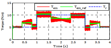
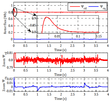
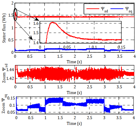
Figure 9 shows the simulation results of Backstepping Control applied to the DFIM tested by a trapezoidal speed set-point with the application of load torque Tr =10N.m at t=1s. these results indicate that:
The amplitude of stator currents increases in proportion to the machine load. During the evolution of the set-points and in particular during the reversal of the rotation direction, with the variation of the load torque, oscillations are observed at the level of the quantities as shown in Figure (9.f and 9.g).
(a) Rotation speed
(b) Electromagnetic torque
Figure 8. Simulation results with speed step
(a) Rotation speed
(b) Speed error
(c) Electromagnetic torque
(d) Rotor flux
(e) Stator flux
(f) Rotor currents
(g) Stator currents
Figure 9. Simulation results with a trapezoidal
4.2.2 Robustness tests
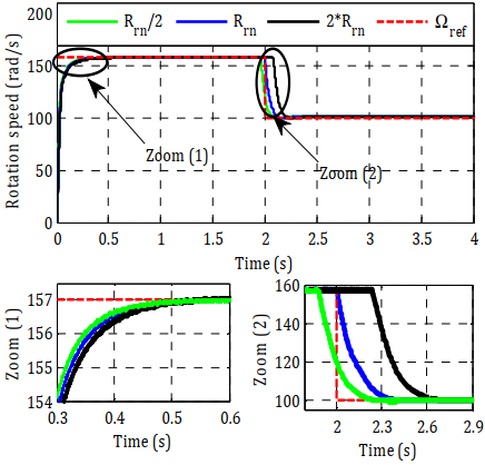
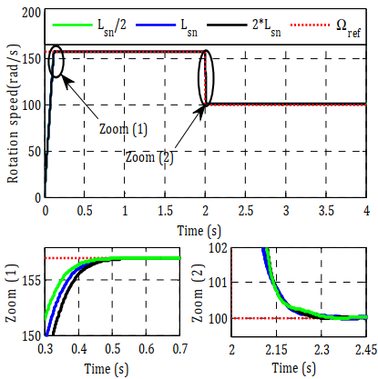
To verify the performance and asymptotic stability of the adaptive Backstepping control on the Rotation Speed, changes are applied to the model parameters of the DFIM used. The results of the simulations are obtained for different robustness tests of the control against parametric variations of the motor, depending on the variation of the resistances (heating cases) and inductances (saturation cases). Figure 10 represent the dynamic behavior of the system in this test.
With regard to robustness to parametric variations, the analysis of the simulation results in Figure 10 shows the superiority of the Backstepping control. Despite these variations, the tracking and regulation behavior remains remarkable. However, a change in the resistance or inductance of its nominal value has no influence on the response time, which remains constant and equal to t=138ms. On the contrary, the rise time changes. The static error of the system is lower. The study of index response indicates that our system remains stable with a response time around the nominal response time without becoming unstable or showing a significant overshoot during parametric variations.
(a) Rotor resistance
(b) Stator resistance
(c) Rotor inductance
(d) Stator inductance
Figure 10. Robustness test for a variation
In order to have a better appreciation of the results obtained, by the two control techniques, a detailed comparative study between these two techniques was realized, in dynamic and static regimes summarizing all the results obtained. This study is done for the same conditions. The Table 2 below summarizes the results of this study.
From this comparison, each control has a set of advantages. The effect of parametric variations on DFIM parameters has been shown along this work to be weaker in the case of adaptive Backstepping control than in the case of rotor flux orientation control. In view of these results, the estimation of the machine parameters provides to the adaptive Backstepping control applied to the DFIM good performances and which exceed the performances of conventional PI regulator.
Table 2. Comparative study between FOC and BACKSTEPPING applied to the DFIM in motor mode
|
FOC |
Adaptive Backstepping |
||
|
Error |
Static |
0.19% |
0.12% |
|
Dynamic |
3% |
0.15% |
|
|
Response time for |
157 rad/s |
271 ms |
138 ms |
|
Trapezoidal speed |
20 ms |
20 ms |
|
|
Overshoot |
157 rad/s |
Null |
Null |
|
Trapezoidal speed |
0.31% |
0.06% |
|
|
Starting torque |
157 rad/s |
17 N.m |
6 N.m |
|
Trapezoidal speed |
2 N.m |
1 N.m |
|
|
Relative drop for 10N.m |
2.54% |
0.255% |
|
|
Rejection time for 10N.m |
100 ms |
70 ms |
|
|
Robustness |
No |
Yes |
|
For this paper, the FOC and Backstepping control strategies for the doubly fed induction motor are presented. The purpose is to make a comparative study between these two control approaches. After testing both techniques using the Matlab/Simulink environment, it concludes that the adaptive Backstepping control offers better performance compared to FOC in terms of static and dynamic error, response time, overshoot and robustness. In addition, another major advantage of the Backstepping control is the insensitivity against parametric changes of the machine. Future work will focus on the implementation of the Backstepping control using an FPGA-based test bench in our laboratory.
|
isd, isq |
Stator currents |
|
ird, irq |
Rotor currents |
|
$\psi_{s d} ,\psi_{s d}$ |
Stator flux (d,q) |
|
$\psi_{r d} ,\psi_{r d}$ |
Rotor flux (d,q) |
|
vsd, vsq |
Stator voltages (d,q) |
|
vrd, vrd |
Rotor voltages (d,q) |
|
Rr, Rs |
Rotor and Stator resistances |
|
Lr, Ls |
Rotor and stator inductance coefficientv |
|
p |
Number of pole pairs |
|
f |
Viscous friction coefficient |
|
σ |
Dispersion coefficient |
|
Msr |
cyclic inductance mutual stator-rotor |
|
ωr |
Electrical angular velocity of the rotor |
|
Ω |
Machine rotation speed |
|
Tem |
Electromagnetic torque |
|
Tr |
Load torque |
|
J |
Moment of inertia |
Parameters of the DFIM
|
Parameter |
Value (unite) |
|
p |
2 |
|
Rs |
1.75 Ω |
|
Rr |
1.68 Ω |
|
Ls |
0.295 H |
|
Lr |
0.104 H |
|
Msr |
0.165 H |
|
J |
0.01 Kg.m² |
|
f |
0.0027 Kg.m²/s |
[1] Bossoufi, B., Karim, M., Lagrioui, A., Taoussi, M., Derouich, A. (2015). Observer backstepping control of DFIG-generators for wind turbines variable-speed: FPGA-based implementation. Renewable Energy, 81: 903-917. https://doi.org/10.1016/j.renene.2015.04.013
[2] Ademi, S., Jovanovic, M. (2014). High-efficiency control of brushless doubly-fed machines for wind turbines and pump drives. Energy Conversion and Management, 81: 120-132. https://doi.org/10.1016/j.enconman.2014.01.015
[3] Babouri, R., Aouzellag, D., Ghedamsi, K. (2013). Introduction of doubly fed induction machine in an electric vehicle. Energy Procedia, 36: 1076-1084. https://doi.org/10.1016/j.egypro.2013.07.123
[4] El Ouanjli, N., Motahhir, S., Derouich, A., El Ghzizal, A., Chebabhi, A., Taoussi, M. (2019). Improved DTC strategy of doubly fed induction motor using fuzzy logic controller. Energy Reports, 5: 271-279. https://doi.org/10.1016/j.egyr.2019.02.001
[5] Blaschke, F. (1972). The principle of field orientation as applied to the new transvector closed-loop system for rotating-field machines. Siemens Review, 34(3): 217-220.
[6] El Ouanjli, N., Derouich, A., El Ghzizal, A., Chebabhi, A., Taoussi, M. (2017). A comparative study between FOC and DTC control of the Doubly Fed Induction Motor (DFIM). In 2017 International Conference on Electrical and Information Technologies (ICEIT), Rabat, pp. 1-6. https://doi.org/10.1109/EITech.2017.8255302
[7] Elmahfoud, M., Bossoufi, B., Taoussi, M., El Ouanjli, N., Derouich, A. (2019). Rotor field oriented control of doubly fed induction motor. 2019 5th International Conference on Optimization and Applications (ICOA), Kenitra, Morocco, pp. 1-6. https://doi.org/10.1109/ICOA.2019.8727708
[8] Profumo, F., DeDoncker, R., Ferraris, P., Pastorelli, M. (1995). Comparison of universal field oriented (UFO) controllers in different reference frames. IEEE Transactions on Power Electronics, 10(2): 205-213. https://doi.org/10.1109/63.372605
[9] Chikhi, A., Djarallah, M., Chikh, K. (2010). A comparative study of fieldoriented control and direct-torque control of induction motors using an adaptive flux observer. Serbian Journal of Electrical Engineering, 7(1): 41-55. https://doi.org/10.2298/SJEE1001041C
[10] Taoussi, M., Karim, M., Bossoufi, B., Hammoumi, D., Lagrioui, A., Derouich, A. (2016). Speed variable adaptive backstepping control of the doubly-fed induction machine drive. Int. J. Automation and Control, 10(1). https://doi.org/10.1504/IJAAC.2016.075140
[11] Zaafouri, A., Regaya, C.B., Azza, H.B., Châari, A. (2016). DSP-based adaptive backstepping using the tracking errors for high-performance sensorless speed control of induction motor drive. ISA Transactions, 60: 333-347. https://doi.org/10.1016/j.isatra.2015.11.021
[12] El Ouanjli, N., Derouich, A., El Ghzizal, A., El Mourabit, Y., Taoussi, M. (2017). Contribution to the improvement of the performances of doubly fed induction machine functioning in motor mode by the DTC control. International Journal of Power Electronics and Drive Systems, 8(3): 1117. https://doi.org/10.11591/ijpeds.v8.i3.pp1117-1127
[13] Zamzoum, O., El Mourabit, Y., Errouha, M., Derouich, A., El Ghzizal, A. (2018). Power control of variable speed wind turbine based on doubly fed induction generator using indirect field‐oriented control with fuzzy logic controllers for performance optimization. Energy Science & Engineering, 6(5): 408-423. https://doi.org/10.1002/ese3.215
[14] Bakouri, A., Mahmoudi, H., Abbou, A. (2016). Intelligent control for doubly fed induction generator connected to the electrical network. International Journal of Power Electronics and Drive Systems, 7(3): 688. http://doi.org/10.11591/ijpeds.v7.i3.pp688-700
[15] Taoussi, M., Karim, M., Hammoumi, D., El Bekkali, C., Bossoufi, B., El Ouanjli, N. (2017). Comparative study between backstepping adaptive and field-oriented control of the DFIG applied to wind turbines. 2017 International Conference on Advanced Technologies for Signal and Image Processing (ATSIP), pp. 1-6. https://doi.org/10.1109/ATSIP.2017.8075592
[16] Bouderbala, M., Bossoufi, B., Lagrioui, A., Taoussi, M., Aroussi, H.A., Ihedrane, Y. (2019). Direct and indirect vector control of a doubly fed induction generator based in a wind energy conversion system. International Journal of Electrical and Computer Engineering, 9(3): 1531. https://doi.org/10.11591/ijece.v9i3.pp1531-1540
[17] Bossoufi, B., Aroussi, H.A., Ziani, E.M., Karim, M., Lagrioui, A., Derouich, A., Taoussi, M. (2014). Robust adaptive backstepping control approach of DFIG generators for wind turbines variable-speed. In 2014 International Renewable and Sustainable Energy Conference (IRSEC), Ouarzazate, pp. 791-797. https://doi.org/10.1109/IRSEC.2014.7059885
[18] Mensou, S., Essadki, A., Minka, I., Nasser, T., Idrissi, B. B. (2017). Backstepping controller for a variable wind speed energy conversion system based on a DFIG. 2017 International Renewable and Sustainable Energy Conference (IRSEC), Tangier, pp. 1-6. https://doi.org/10.1109/IRSEC.2017.8477586
[19] Farhani, F., Regaya, C.B., Zaafouri, A., Chaari, A. (2017). Real time PI-backstepping induction machine drive with efficiency optimization. ISA Transactions, 70: 348-356. https://doi.org/10.1016/j.isatra.2017.07.003
[20] Abdelghafour, H., Abderrahmen, B., Samir, Z., Riyadh, R. (2018). Backstepping control of a doubly-fed induction machine based on fuzzy controller. European Journal of Electrical Engineering, 20(5-6): 645-657. https://doi.org/10.3166/EJEE.20.645-657