Image Processing Techniques for Dynamic Surface Velocity Measurement in Rivers

The traditional Mean shift algorithm exhibits noticeable limitations in tracking river surface targets. Typically employing a single statistical feature modeling, such as color histograms, to represent the target model, the algorithm struggles with the complex and variable river surface environments. Factors such as lighting conditions, surface reflections, and wave changes easily affect the stability of color features, rendering the algorithm ineffective in accurately capturing and tracking targets. Moreover, the limited descriptive capability of a single feature often leads to tracking failure when target morphology changes or when the background features resemble those of the target. To address these deficiencies, an improved Mean shift algorithm that integrates grayscale statistical features with Histogram of Oriented Gradients (HOG) features is proposed. This hybrid model retains the non-parametric search advantages of the original Mean shift algorithm while enhancing target morphology and structural information extraction capabilities through the inclusion of HOG features, thereby effectively enriching and bolstering target representation robustness. Grayscale features exhibit strong robustness to lighting variations, and HOG features are sensitive to target edges and shapes. The combination of these significantly improves the algorithm's tracking performance in complex water surface environments. Assuming the gradients of point (a,b) in the horizontal and vertical directions are represented by H_a(a,b) and H_b(a,b), respectively, the process of calculating the HOG features is as follows:

$\begin{align}  & {{H}_{a}}\left( a,b \right)=U\left( a+1,b \right)-U\left( a-1,b \right)  & {{H}_{b}}\left( a,b \right)=U\left( a,b+1 \right)-U\left( a,b-1 \right) \end{align}$                   (1)

Based on the aforementioned calculations, the gradient magnitude and direction at point (a,b) can be further determined using the following formula:

$\begin{align}  & H\left( a,b \right)=\sqrt{{{H}_{a}}{{\left( a,b \right)}^{2}}+{{H}_{b}}{{\left( a,b \right)}^{2}}} & \beta \left( a,b \right)=ARCTAN\left( \frac{{{H}_{a}}\left( a,b \right)}{{{H}_{b}}\left( a,b \right)} \right) \end{align}$                       (2)

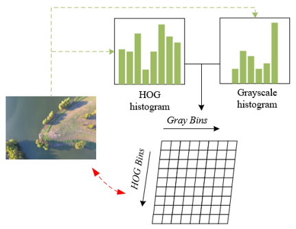
In the context of this study on dynamic river surface velocity measurement, it is crucial to construct an accurate target tracking model to ensure measurement accuracy and reliability under various environmental conditions. Initially, for a given river surface image area, preprocessing steps are employed to optimize the image for better feature extraction. Preprocessing includes noise reduction and contrast enhancement, among other steps, to mitigate the impacts of environmental noise and lighting variations. Subsequently, two parallel feature extraction operations are performed on the preprocessed image area: calculation of the grayscale histogram and extraction of HOG features. The grayscale histogram is constructed by tallying the frequency of each gray level present in the image, providing information on the distribution of image brightness. The process of extracting HOG features involves calculating the gradient direction and intensity in local areas of the image. Figure 1 illustrates the construction of the target model integrating grayscale and HOG features.

1.png

Figure 1. Schematic for establishing a target model integrating grayscale and HOG features

2.png

Figure 2. Basic principle of the Meanshift algorithm

Following the extraction, the grayscale histogram and HOG feature vectors undergo normalization to eliminate disparities between different feature magnitudes, ensuring their comparability during subsequent integration. Subsequently, the two normalized feature vectors are merged into a unified feature space to construct the final target description model. This process is based on the joint probability distribution, specifically estimated through a statistical method that assesses the joint distribution of the two features. Assuming the normalized pixel position centered on the target is represented by c*_u, with the target center coordinates denoted by (a₀,b₀), the grayscale value at pixel position c_uk within the target area's interval index value in the grayscale histogram is indicated by β(c_uk), and the HOG value at pixel position c_uk within the target area's interval index value in the HOG histogram is represented by α(c_uk). The interval index value vector divided by the grayscale histogram is denoted by i, and the interval index value vector divided by the HOG histogram is denoted by n. The target model expression is provided as follows:

$w=z\sum\limits_{u=1}^{l}{\sum\limits_{k=1}^{v}{J\left( ||c_{u}^{*}|{{|}^{2}} \right)}\sigma \left[ \beta \left( {{c}_{uk}}-i \right) \right]\sigma \left[ \alpha \left( {{c}_{uk}} \right)-v \right]n}$                     (3)

where,

$\begin{align}  & z=\frac{1}{\sum\limits_{u=1}^{l}{\sum\limits_{k=1}^{v}{J\left( ||c_{u}^{*}|{{|}^{2}} \right)}}} \\ & c_{u}^{*}={{\left( \frac{{{\left( {{a}_{uk}}-{{a}_{0}} \right)}^{2}}+{{\left( {{b}_{uk}}-{{b}_{0}} \right)}^{2}}}{a_{0}^{2}+b_{0}^{2}} \right)}^{\frac{1}{2}}} \\\end{align}$                     (4)

Based on this model, the iterative search process of the Meanshift algorithm is utilized to identify and locate dynamically changing candidate regions within continuous video frames. Figure 2 illustrates the basic principle schematic of the Meanshift algorithm. In each iteration, by calculating the similarity between the current candidate area and the original model, combined with the method of probability distribution, the search window is dynamically adjusted to adapt to the movement and morphological changes of the target on the river surface. Thus, the description template of each candidate area is updated in real-time, accurately capturing the latest state of the target. The center position of the candidate target is denoted by d, and the size of the kernel function window is represented by g. The expression for the description template o of the corresponding candidate target area is given as follows:

$o=z\sum\limits_{u=1}^{l}{\sum\limits_{k=1}^{v}{J\left( {{\left\| \frac{d-{{c}_{uk}}}{g} \right\|}^{2}} \right)}}\sigma \left[ \beta \left( {{c}_{uk}} \right)-i \right]\sigma \left[ \beta \left( {{c}_{uk}} \right)-n \right]$                 (5)

The Meanshift iteration process for the specific river surface target tracking algorithm includes defining the Bhattacharyya coefficient. In the context of target tracking, W represents the feature distribution based on the target model, while O represents the feature distribution of the candidate target area. With the use of fused variables, the definition is as follows:

$\vartheta \left( O,W \right)=\sum\limits_{u=1}^{l}{\sum\limits_{k=1}^{v}{\sqrt{{{o}_{uk}}{{w}_{uk}}}}}$                (6)

To simplify the calculation, the Bhattacharyya coefficient is expanded using Taylor series to obtain its approximate expression:

$\vartheta \left( o,w \right)\approx \frac{1}{2}\sum\limits_{u=1}^{l}{\sum\limits_{k=1}^{v}{\sqrt{o\left( {{d}_{0}} \right)w}}+\frac{Z}{2}\sum\limits_{u=1}^{l}{\sum\limits_{k=1}^{v}{o\left( d \right)}\sqrt{\frac{w}{o\left( {{d}_{0}} \right)}}}}$                  (7)

The core objective of the Meanshift iteration equation is to maximize the approximation of the Bhattacharyya coefficient, thereby making the feature distribution of the candidate area as similar as possible to the feature distribution of the target model. In each iteration, by calculating the Bhattacharyya coefficient between the current candidate area and the target model, then moving the center of the candidate area to maximize this coefficient. The direction of movement is determined by the difference between the current position and the probability centroid. This iterative process continues until convergence is reached, that is, when the candidate area no longer undergoes significant changes, or the increment of the Bhattacharyya coefficient is below a certain threshold. The statistical value of the grayscale index u and HOG index k in the candidate template is denoted by w_uk, and the statistical value of the grayscale index u and HOG index k in the target template is denoted by O_uk. The corresponding iterative equations are provided as follows:

${{d}_{j+1}}={{d}_{j}}+\frac{\sum\limits_{u=1}^{l}{\sum\limits_{k=1}^{v}{{{\mu }_{uk}}\left( {{d}_{j}}-{{c}_{uk}} \right)}h\left( \left\| \frac{{{d}_{j}}-{{c}_{uk}}}{g} \right\| \right)}}{\sum\limits_{u=1}^{l}{\sum\limits_{k=1}^{v}{{{\mu }_{uk}}h\left( \left\| \frac{{{d}_{j}}-{{c}_{uk}}}{g} \right\| \right)}}}$              (8)

${{\mu }_{uk}}=\sum\limits_{u=1}^{8}{\sum\limits_{k=1}^{9}{\sqrt{\frac{{{w}_{uk}}}{{{o}_{uk}}\left( d \right)}}\sigma \left[ \beta \left( {{c}_{uk}} \right)-i \right]\sigma \left[ \alpha \left( {{c}_{uk}} \right)-n \right]}}$               (9)

Hu invariant moments, as shape descriptors, provide crucial characteristic information about the shape of target objects, which remains invariant for target identification and tracking, even under image scaling, rotation, or reflection, thus maintaining consistency. This study opts to integrate Hu invariant moments with template similarity coefficients to establish new iterative convergence criteria. By incorporating template similarity coefficients, a more comprehensive assessment of the similarity between the candidate and model targets can be achieved. This assessment encompasses not only features such as grayscale and texture but also shape information unaffected by changes in viewpoint. Such iterative convergence criteria aid in enhancing the adaptability and robustness of the river surface target tracking algorithm in complex environments. It ensures that, even under complex conditions like surface reflection and wave changes, targets can still be accurately captured and tracked, thereby providing stable and reliable data support for velocity measurement. This study defines the following seven Hu moments:

$\begin{align}  & {{g}_{1}}={{\lambda }_{20}}+{{\lambda }_{02}} \\ & {{g}_{2}}={{({{\lambda }_{20}}-{{\lambda }_{02}})}^{2}}+4\lambda _{11}^{2} \\ & {{g}_{3}}={{\left( {{\lambda }_{30}}-3{{\lambda }_{12}} \right)}^{2}}+{{\left( 3{{\lambda }_{21}}-{{\lambda }_{03}} \right)}^{2}} \\ & {{g}_{4}}={{\left( {{\lambda }_{30}}+{{\lambda }_{12}} \right)}^{2}}+{{\left( {{\lambda }_{21}}+{{\lambda }_{03}} \right)}^{2}} \\ & {{g}_{5}}=\left( {{\lambda }_{30}}-{{\lambda }_{12}} \right)\left( {{\lambda }_{30}}+{{\lambda }_{12}} \right)\left[ {{\left( {{\lambda }_{30}}+{{\lambda }_{12}} \right)}^{2}}-3{{\left( {{\lambda }_{21}}+{{\lambda }_{03}} \right)}^{2}} \right] \\ & +\left( 3{{\lambda }_{21}}-{{\lambda }_{03}} \right)\left( {{\lambda }_{21}}+{{\lambda }_{03}} \right)\left[ 3{{\left( {{\lambda }_{30}}+{{\lambda }_{12}} \right)}^{2}}-{{\left( {{\lambda }_{21}}+{{\lambda }_{03}} \right)}^{2}} \right] \\ & {{g}_{6}}=\left( {{\lambda }_{20}}-{{\lambda }_{02}} \right)\left[ {{\left( {{\lambda }_{30}}+{{\lambda }_{12}} \right)}^{2}}-{{\left( {{\lambda }_{21}}+{{\lambda }_{03}} \right)}^{2}} \right]+4{{\lambda }_{11}}\left( {{\lambda }_{30}}+{{\lambda }_{12}} \right)\left( {{\lambda }_{21}}+{{\lambda }_{03}} \right) \\ & {{g}_{7}}=\left( 3{{\lambda }_{21}}-{{\lambda }_{03}} \right)\left( {{\lambda }_{30}}+{{\lambda }_{12}} \right)\left[ {{\left( {{\lambda }_{30}}+{{\lambda }_{12}} \right)}^{2}}-3{{\left( {{\lambda }_{21}}+{{\lambda }_{03}} \right)}^{2}} \right] \\ & +\left( 3{{\lambda }_{12}}-{{\lambda }_{03}} \right)\left( {{\lambda }_{21}}+{{\lambda }_{03}} \right)\left[ 3{{\left( {{\lambda }_{30}}+{{\lambda }_{12}} \right)}^{2}}-{{\left( {{\lambda }_{21}}+{{\lambda }_{03}} \right)}^{2}} \right] \\\end{align}$           (10)

Assuming the candidate and target models based on fused grayscale and HOG features are represented by O_i and W_i, respectively, and the Hu moment vectors of the candidate and target models are denoted by O_g and W_g, the Euclidean distance between Hu invariant moment vectors is represented by DI(O_g(d)W_g). Taking into consideration both the Hu invariant moments and the similarity coefficients between O_i and W_i, the expression for the algorithm's convergence criterion is provided as follows:

$\vartheta =MAX\left( \sqrt{{{o}_{i}}\left( d \right){{W}_{i}}} \right)\hat{\ }MIN\ DI\left( {{P}_{g}}\left( d \right){{w}_{g}} \right)$                   (11)

The process steps of the river surface target tracking algorithm based on the improved Meanshift are detailed as follows, as depicted in Figure 3:

(a) At the initiation stage of measuring the dynamic surface velocity of the river, the first frame of the video sequence is acquired. Through the method of differencing, this step effectively separates moving targets from the background, further calculating the target area markers to indicate the initial position and size of the target.

(b) Based on the position of the target, the Region of Interest (ROI) is cropped. Within this area, the Hu invariant moment vector, as well as the grayscale histogram and the orientation gradient histogram vector of the ROI, are calculated. These features, together with the Hu moment vector, constitute the description template of the target.

(c) The next frame image is read, and the candidate target area corresponding to the previously located ROI is cropped. The description template for this candidate area, including the Hu moment vector and its weight matrix, is calculated, and based on this, the next possible position of the target is determined. The weight matrix is calculated based on the feature distribution within the candidate area, reflecting the contribution of different pixels to target localization.

(d) The similarity between the ROI and the candidate area is evaluated by calculating the Bhattacharyya coefficient between them. Additionally, the similarity between their Hu invariant moment vectors is measured using the Euclidean distance. By combining these two similarity indices, the proximity between the candidate area and the true target area can be more accurately judged.

(e) If both the Bhattacharyya coefficient and the similarity of the Hu vectors reach the threshold set by the algorithm, it can be concluded that the optimal position of the target in the current frame has been found. If the predetermined threshold is not reached, the algorithm continues the iterative search until convergence.

Once the optimal position of the target is determined, the area of the target in the current frame is calculated using the region growing method. At this step, it is necessary to decide whether to update the target description template to adapt to possible changes in the target during motion. Meanwhile, the Bhattacharyya coefficient is calculated, and whether to update the model is judged based on the preset threshold. If an update is required, the algorithm returns to the second step, recalculating the ROI and the target description template.

(f) The algorithm determines whether all frames have been processed. If not, the third step is continued with the processing of the next frame image. If all frames have been processed, the algorithm concludes.

3.png

From Table 1, it is observed that for a 15*20 river surface target subjected to various transformations, the calculated Hu values were obtained. According to the theory of Hu invariant moments, these transformations should not significantly alter the Hu values. The data in the table indicate that for g₁, the Hu values remain close under different transformations, demonstrating the consistency of g₁ through these changes and proving its invariance. For g₂ to g₇, although numerical values changed following translation, rotation, and scaling operations, the extent of change is generally small, which to some extent supports the stability of Hu invariant moments. Notably, the changes in g₃ and g₄ are very minimal, indicating these moments are particularly stable against rotation and scaling. It is important to note that while Hu invariant moments possess invariance to these operations, due to limitations in calculation and representation accuracy, especially in digital image processing, theoretical invariance may manifest as approximate invariance in practical applications, which could be one of the reasons for the slight variations in Hu values. The invariance of Hu values to flipping, as well as subsequent rotation and scaling, especially the values of g₁, indicates that these moments are stable against such transformations. Integrating Hu invariant moments as image features for river surface target tracking technology studied in this article is reasonable. Through the improved Meanshift algorithm, these Hu invariant moments can be used as template matching features within the tracking algorithm to enhance the identification and tracking capabilities of dynamic water surface targets. In complex environments, even as targets undergo transformations such as rotation, scaling, or flipping, Hu invariant moments provide stable features for the algorithm, thereby aiding in the accurate tracking of targets, which is especially important in dynamic and variable river environments. Furthermore, combining similarity coefficients with templates can further enhance the robustness of the algorithm, ensuring stability and reliability in the tracking process in practical applications.

Comparing the tracking accuracy of various algorithms on both the training and testing sets, as illustrated in Figure 6, for different centroid error thresholds, it can be concluded that the algorithm proposed in this study exhibits slightly higher accuracy compared to deep learning based Simple Online and Realtime Tracking (DeepSORT), and significantly outperforms You Only Look Once (YOLO) and Mask Region-Convolutional Neural Network (R-CNN) on both the training and testing sets. This indicates that the improved Meanshift algorithm provides stable tracking performance, especially maintaining high accuracy even with larger centroid errors. The river surface target tracking method based on the improved Meanshift algorithm demonstrates excellent stability on the training set and good generalization capabilities on the testing set. This suggests that the algorithm proposed in this study is better adapted to changes in targets, especially in complex dynamic environments, providing stable and accurate tracking results. Therefore, the algorithm proposed in this study is effective and valuable for river surface target tracking tasks.

Analyzing the processing time of different algorithms for river surface image sequences as shown in Table 2, the following conclusions can be drawn: The algorithm proposed in this study demonstrates a significant advantage in processing time, especially when compared to the computationally intensive DeepSORT and Mask R-CNN. Even when compared to YOLO, the proposed algorithm exhibits competitive processing speeds in most cases and is faster in certain sequences. This aspect is critically important for scenarios requiring real-time or rapid processing, such as river surface target tracking, which may necessitate swift responses to ensure navigational safety or conduct environmental monitoring. The river surface target tracking method based on the improved Meanshift algorithm not only excels in tracking accuracy but also shows superiority in processing time. The low latency of processing times makes this method particularly effective for real-time applications that require quick responses. Therefore, the algorithm proposed in this study is not only technically feasible but also valuable in practical applications, especially in environments where resources are limited or where time sensitivity is crucial.

61.png

(a) Training set

62.png

(b) Testing set

Figure 6. Comparison of tracking accuracy of different algorithms for river surface targets

Table 1. Hu values for a 15*20 river surface target after various transformations

Table 2. Processing time of different algorithms for river surface image sequences

Table 3. Comparison of results using different dynamic river surface flow velocity measurement methods

Table 4. Comparison of dynamic river surface flow velocity measurement results across different distances

Table 5. Comparison of dynamic river surface flow velocity measurement results for multiple sections at the same distance