Naaman Omar![]()
© 2024 The author. This article is published by IIETA and is licensed under the CC BY 4.0 license (http://creativecommons.org/licenses/by/4.0/).
OPEN ACCESS
Autism Spectrum Disorder (ASD) is a complex condition affecting children and characterized by challenges in social interaction, communication, and behavior. Typically, evident before the age of three, ASD severity varies. Diagnosis involves a thorough assessment by a multidisciplinary team using criteria from the Diagnostic and Statistical Manual of Mental Disorders, Fifth Edition (DSM-5), a comprehensive guide for mental health conditions, including ASD. This study focuses on employing deep learning techniques and electroencephalogram (EEG) signals for ASD detection. A unique approach is introduced, utilizing a multi-input 1D Convolutional Neural Network (CNN) framework. EEG signals undergo processing, and data augmentation using sliding windows precedes input into the multi-input 1D CNN model. This model incorporates various layers, including 1D convolutional layers, batch normalization, ReLU activation, and a fully connected layer. Experiments utilize EEG data from King Abdulaziz University Hospital, and the method's effectiveness is evaluated using diverse performance metrics. The experimental work is structured into three sections. The initial experiment focuses on specific EEG channels (FP1, FP2, F7, F3, Fz, F4, and F8), achieving a remarkable accuracy of 99.16%. Expanding the investigation to central and temporal EEG channels (C4, Cz, C3, T5, and Pz) yields an accuracy of 98.32%. In the final experiment involving occipital channels (O1, Oz, O2), an accuracy of 97.65% is achieved. Comparative analyses with existing methods consistently demonstrate the superior performance of our proposed approach.
Autism Spectrum Disorder, EEG signals, multi-input CNN model, EEG channels, deep learning
Autism Spectrum Disorder (ASD) in children is a complex neurodevelopmental condition characterized by a spectrum of challenges in social interaction, communication, and behavior [1]. It typically manifests early in a child's development, often becoming evident by the age of three [2]. Children with ASD exhibit a wide range of symptoms, with some displaying severe impairments in language development, social engagement, and repetitive behaviors, while others may have milder symptoms and unique strengths. The diagnosis of ASD in children is based on careful observation of their behavior and developmental milestones, often involving assessments by a multidisciplinary team of clinicians, including psychologists, speech therapists, and pediatricians [3]. The underlying causes of ASD in children remain a subject of ongoing research, with evidence suggesting a complex interplay of genetic, environmental, and neurological factors. Early intervention is critical in addressing the unique needs of children with ASD, as it can significantly improve their developmental outcomes and quality of life [4]. Tailored interventions may include speech and language therapy, applied behavior analysis, sensory integration therapy, and educational support. Additionally, promoting awareness and understanding of ASD among parents, educators, and the community at large is essential in fostering an inclusive and supportive environment for children with ASD, enabling them to thrive and reach their full potential. The World Health Organization (WHO) reports that approximately one in every 160 children is impacted by ASD [5]. Although there is currently no cure for ASD, early intervention is deemed essential as it significantly contributes to enhancing social skills, communication abilities, and cognitive development. Consequently, the development of a dependable, efficient, and accurate diagnostic method for ASD holds paramount importance [6]. ASD is intricately tied to neurobiological factors, demonstrated by studies exploring its neuroscience and medical basis. Brain structural anomalies, such as enlarged frontal and temporal lobes, alongside irregularities in regions like the amygdala and cerebellum, characterize its neural correlates. Connectivity disruptions affecting both short- and long-range neural pathways contribute to processing and integration challenges. The mirror neuron system, vital for understanding and imitating actions, is implicated in ASD, with potential dysfunction noted. A strong genetic component, involving genes related to synaptic function and neuronal development, underlies the disorder. The heterogeneity of ASD points to a complex interplay of genetic and non-genetic factors, emphasizing its intricate medical basis. Advances in neuroscience deepen our understanding, guiding targeted interventions and therapies.
Current ASD diagnostic methods have limitations, such as reliance on subjective observations and a shortage of specialists leading to delays. AI aims to enhance accuracy and efficiency by providing standardized assessments and mitigating subjectivity. AI tools can expedite diagnoses through quick analysis of large datasets and address the heterogeneity of ASD by capturing diverse symptoms. This has the potential to revolutionize ASD diagnosis, making it more precise, timely, and personalized.
The diagnostic process for ASD employs a comprehensive approach, incorporating clinical observations, standardized assessments, and behavioral evaluations. Healthcare professionals and specialists utilize a variety of diagnostic tools and methodologies to evaluate both the presence and severity of ASD symptoms in individuals. Noteworthy among these tools are the Autism Diagnostic Observation Schedule (ADOS), a standardized observational assessment designed to scrutinize social and communicative behaviors, and the Autism Diagnostic Interview-Revised (ADI-R), an extensive caregiver interview focused on gathering information about a child's developmental history and behavioral patterns. In addition to these tools, developmental assessments such as the Modified Checklist for Autism in Toddlers (M-CHAT) function as valuable screening instruments, especially for young children, helping identify potential indicators of ASD. These assessments are often complemented by advanced neuroimaging techniques, including Magnetic Resonance Imaging (MRI) and Electroencephalography (EEG), which aim to explore potential underlying neurological correlates associated with ASD. The integration of these multifaceted diagnostic tools and approaches is of paramount importance in ensuring the accurate and timely diagnosis of ASD, a crucial step that facilitates access to tailored interventions and support for individuals with ASD.
EEG for ASD detection has a lower spatial resolution compared to MRI. EEG measures electrical activity on the scalp, providing information about overall brain function, but it may lack the precision to pinpoint specific brain regions involved in ASD. In contrast, MRI offers higher spatial resolution, allowing for detailed imaging of brain structures and potential abnormalities.
The utilization of EEG in ASD detection involves capturing and analyzing electrical brain activity to identify specific patterns or irregularities associated with ASD. This non-invasive neuroimaging technique provides valuable insights into the neural signatures and functional connectivity of individuals with ASD, contributing to both early diagnosis and ongoing research into the condition. Ari et al. [7] introduced an innovative approach for ASD detection via EEG recordings. They employed the Douglas-Peucker algorithm to initially reduce sample size per channel without degrading EEG quality. Next, EEG rhythms were extracted using the wavelet transform and represented sparsely through the matching pursuit algorithm. An image was constructed by merging histograms of these processed rhythm signals. Data augmentation included Extreme Learning Machines-based autoencoders. Following augmentation, pre-trained deep CNN models were used to classify ASD and healthy EEG signals, achieving a 98.88% accuracy. In their study, Patel et al. [8] introduced a novel CNN-based feature extractor for the brain-computer interface attention classification framework. The proposed model included a feature extractor architecture and a subsequent shallow classifier, which facilitated precise classification of the responses of ASD patients to stimuli. Upon evaluating the model's performance using standard metrics such as the confusion matrix, accuracy, and F1 scores, it was observed that the model achieved an impressive accuracy rate of 91%. Tawhid et al. [9] conducted a comprehensive study for ASD detection, utilizing both traditional machine learning and deep learning approaches. They extracted textural features and conducted feature selection with principal component analysis, employing six machine-learning classifiers alongside three distinct CNN models. Remarkably, their deep learning approach achieved an impressive 99.15% accuracy on an EEG dataset related to ASD, while the machine-learning model yielded a commendable 95.25% accuracy. Peya et al. [10] introduced an EEG-based approach utilizing CNNs, converting individual EEG channel data into 2D images through Pearson's correlation coefficient. Their CNN model with residual connections achieved an exceptional classification accuracy of 100% on clinical EEG data. Xu et al. [11] aimed to distinguish children with ASD from those without using short-term hemodynamic fluctuations, employing a multilayer neural network combining CNN with a gated recurrent unit. Tested on an EEG dataset comprising 25 ASD and 22 non-ASD subjects, this integrated model achieved an impressive accuracy of 92.2%. Loganathan et al. [12] introduced a hybrid ensemble model combining ResNet101 with a bidirectional gated recurrent unit (Bi-GRU) through a weighted average ensemble. Their preprocessing phase, which filtered out unwanted elements, coupled with a ResNet-based CNN for classification, resulted in remarkable accuracy, reaching 98%. In a comprehensive review, Sharifi et al. [13] evaluated various EEG and machine learning-based ASD detection methodologies, assessing algorithms, strengths, and limitations. The review emphasized the crucial role of preprocessing techniques, feature extraction, and selection methods applied to EEG data, as well as the selection of classifiers in determining classification accuracy. Notably, among the learning-based approaches, CNNs emerged as the preferred choice due to their demonstrated capability to achieve superior levels of accuracy.
The existing literature reveals a notable shift in research on ASD detection using EEG and artificial intelligence, with a growing emphasis on deep learning. In response to this trend, our study introduces a novel approach for EEG-based ASD detection, utilizing a multi-input 1D CNN framework. Prior to analysis, EEG signals underwent preprocessing, including band-pass filtering to eliminate noise. A crucial step involved data augmentation through an overlapping sliding window technique, effectively segmenting the time-domain EEG signal. In this process, each EEG channel served as an individual input to the multi-input 1D CNN model, aligning with the channel count of the EEG signal. The constructed model consisted of two convolutional layers, each followed by batch normalization and Rectified Linear Unit (ReLU) activation functions. A flatten layer processed the output of the activation layer, and the results from all flatten layers were concatenated and directed into a fully connected layer. The model was finalized with a softmax layer and a classification output layer, forming the proposed multi-input 1D CNN architecture. The EEG dataset, sourced from King Abdulaziz University Hospital, formed the basis for our experimental investigations [14]. To evaluate the proposed method's effectiveness, various performance metrics were employed. The primary contributions of this paper are twofold: firstly, the utilization of EEG channel signals as inputs to a multi-input 1D CNN model, which, to the best of our knowledge, is a novel approach; secondly, the achievement of significantly higher accuracy scores for the examined dataset.
The structure of the paper unfolds as follows: Section 2 delves into a detailed exposition of the materials and methodologies employed. Section 3 provides a comprehensive overview of the experimental procedures and ensuing results. In Section 4, extensive discussions regarding the findings are presented. Finally, Section 5 succinctly encapsulates the conclusions drawn from the study and outlines potential avenues for future research.
In this section, the related materials and methods are given to carry out the EEG-based ASD detection where each channel of the EEG signal is used as input to the multi-input 1D CNN model [15-17]. Figure 1 shows the illustration of the proposed method.
Figure 1. Illustration of the proposed method
As depicted in Figure 1, the model architecture incorporates a series of one-dimensional convolutional layers, each responsible for processing an individual channel signal. After the initial convolutional layer, the model employs batch normalization and Rectified Linear Unit (ReLU) layers. Following the first ReLU layer, another set of three layers, comprising convolution, batch normalization, and ReLU layers, is sequentially arranged. The final ReLU layers' outputs are subjected to flattening and concatenation to form an input structure for the fully connected layer. To finalize the model architecture, softmax, and classification output layers are employed. The model is trained utilizing the 'Adam' optimization algorithm.
2.1 Data augmentation
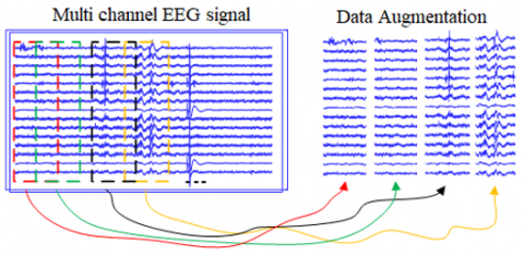
Data augmentation of EEG signals can be achieved through the implementation of an overlapping sliding window technique [18]. In this method, the continuous EEG signal is divided into fixed-length windows or segments, which serve as the fundamental units for analysis or machine learning model training. To introduce variability and capture temporal dependencies, these windows overlap with each other, meaning that certain sections of adjacent windows share common EEG data [19]. The degree of overlap, typically specified as a percentage of the window size, can be adjusted to control the level of augmentation. This strategy demonstrates its utility across a range of EEG applications, including tasks like categorizing brain states or detecting disorders. It empowers the model to capture finer-grained features and temporal patterns from the data, enhancing its effectiveness in these applications. Moreover, overlapping sliding windows find utility in time-frequency analysis, facilitating the exploration of frequency components over time. However, the choice of window size and overlap percentage is application-dependent and may require experimentation to optimize the data augmentation process for a specific EEG analysis task, ultimately enhancing the robustness and performance of the analysis or machine learning model. Figure 2 shows an illustration of an overlapping sliding window method.
Figure 2. Data augmentation procedure
2.2 The dataset
The dataset utilized in this investigation was sourced from the King Abdulaziz University Hospital in Jeddah, Saudi Arabia [14]. It comprises 20 children diagnosed with ASD, aged between 6 and 20 years. Additionally, a control group consisting of nine children with no history of neurological conditions was included for comparison. EEG signals were recorded from participants in a relaxed state using a G-tec EEG cap equipped with Ag/AgCl electrodes, G-tech USB amplifiers, and BCI2000 software, ensuring the acquisition of artifact-free EEG data. The data collection involved recordings from 16 channels (FP1, FP2, F7, F3, Fz, F4, F8, T3, C4, Cz, C3, T5, Pz, O1, Oz, and O2) following the international 10–20 systems configuration, with AFz serving as the ground reference and the right ear lobe as specified in [20]. It's essential to highlight that this dataset is publicly accessible, and all requisite ethical approvals were obtained [14]. The architecture referred to as "-18" denotes a deep CNN architecture with 18 layers.
2.3 Multi-input 1D CNN
A CNN stands as a profound architecture in the realm of machine learning, particularly influencing tasks related to image analysis and recognition [14, 20, 21]. CNNs are composed of multiple layers, encompassing convolutional layers, pooling layers, and fully connected layers, collaboratively designed to progressively extract and process features from the input data. Convolutional layers employ learnable filters to convolve over the input, enabling the network to discern and identify local patterns. Pooling layers then down sample the feature maps, reducing spatial dimensions and computational complexity. Lastly, fully connected layers amalgamate the extracted features to make predictions or classifications. This architecture has proven transformative in various applications, solidifying its significance in the field.
In this paper, as the input is a signal, a one-dimensional convolution layer is employed at the beginning of the developed model [15]. The convolution operation for a 1D signal in a CNN involves applying a convolutional layer to the input signal using a set of learnable filters or kernels. The 1D convolution operation for each filter k is computed as follows:
$y^k[n]=\sum_{m=0}^{M-1} W^k(m) \cdot x(n-m)$ (1)
In the above equation, n represents the current position in the output map yk. m is the position within the filter Wk, ranging from zero to M-1. x(n-m) corresponds to the element of the input signal x at position m-n. Wk(m) represents the filter coefficient at position m for filter k. This operation is applied independently to each filter k, resulting in a set of output feature maps y1,y2,…,yk. These feature maps are then typically passed through an activation function to introduce non-linearity and form the final output of the convolutional layer. Batch normalization is a technique utilized to standardize the outputs of individual layers within a neural network model. In the training phase, this method calculates a scaling factor to transform the mean to zero and the variance to one for each batch of data. Following this standardization, the outputs undergo activation functions. Mathematically, batch normalization can be described by the following equations:
$\mu_B=\frac{1}{m} \sum_{i=1}^m x_i$ (2)
$\sigma_B^2=\frac{1}{m} \sum_{i=1}^m\left(x_i-\mu_B\right)^2$ (3)
$\hat{x}_i=\frac{x_i-\mu_B}{\sqrt{\sigma_B^2+\epsilon}}$ (4)
$y_i=\gamma \hat{x}_i+\beta$ (5)
In the provided equations, xi represents the i-th example within a batch, $\mu_B$ denotes the batch mean, and $\sigma_B^2$ stands for the batch variance. $\hat{x}_i$ represents the normalized output. γ and β are the scale factor and bias parameters, respectively. ϵ is a small value introduced to prevent division by zero errors. These equations illustrate the process of first computing the batch mean and variance, then utilizing these values to obtain the normalized output, and finally applying the scale factor and bias terms. This operation can be applied to normalize the output of any layer within a neural network model. Batch normalization often contributes to a faster and more stable training process, thereby enhancing the overall performance of neural networks.
The Rectified Linear Unit (ReLU) is a widely used activation function in neural network models. The ReLU function outputs the input value directly if it is greater than zero, and assigns an output value of zero if the input is less than zero [21]. Mathematically, the ReLU function is expressed as follows:
$f(x)=\max (0, x)$ (6)
In this equation, x represents the input value, and f(x) represents the output value. The graph of the function exhibits a value of zero on the x-axis for negative input values and rises linearly with a slope of x for positive input values. The ReLU function can be employed as the activation function for any layer within a neural network model. Notably, in deep neural network models, utilizing the ReLU function helps mitigate the problem of vanishing gradients for input values near zero, resulting in faster learning.
The flattening layer is a layer within a neural network model that transforms the output of any preceding layer into a single vector. This layer is commonly used, especially in the processing of image inputs. The flattening layer can be expressed mathematically by the following equation:
flatten $(X)=X^{\prime}$ (7)
In this context, X represents a tensor that comes from the previous layer, while X' refers to the tensor that has been flattened or transformed into a one-dimensional vector. The Concatenation layer is a layer that combines two or more tensors to create a new tensor. This layer is particularly useful in neural network models when there is a need to merge multiple pathways or when input data has distinct features. Mathematically, the Concatenation layer can be expressed using the following equation:
$\operatorname{concat}\left(X_1, X_2, \ldots, X_n\right)=\mathrm{Y}$ (8)
Here, $X_1, X_2, \ldots, X_n$ represent the tensors to be concatenated, and Y is the resulting tensor. The numbers $1,2, \ldots, n$ respectively indicate the number of channels in each tensor. A FC Layer, alternatively referred to as a Dense Layer, is a neural network layer designed to process vectorized input data and generate an output vector through matrix multiplication. Typically employed in the concluding layers of a neural network, this layer produces outputs utilized in tasks like classification or regression. The mathematical expressions governing a FC Layer are outlined below:
$y=\sigma(W x+b)$ (9)
In this context, x is an n-dimensional vector representing the input to the layer. W is the weight matrix with dimensions m×n, where m represents the size of the output vector. b is the bias term, a vector of size m. σ is the activation function. The Softmax layer is an output layer commonly used in classification problems. It interprets the input vector data as probabilities belonging to different classes and selects the most likely class. The Softmax function calculates the probability of each class by normalizing the individual class scores concerning the total probabilities. The mathematical equations for the Softmax layer are as follows:
$y_i=\frac{e^{z_i}}{\sum_{j=1}^C e^{z_j}}$ (10)
Here, $y_i$ represents the probability of the ith class, and $Z_i$ is the net output value for the ith class. C is the total number of classes. The Softmax function calculates the ratio of $e^{z_i}$ contributing to the total probability of class C to $e^{z_i}$, where $Z_i$ is the net output for class i. Consequently, the probability of each class is normalized relative to the sum of $e^{z_i}$ divided by C. Consequently, the sum of probabilities assigned to all classes by the Softmax function always equals one. Another noteworthy characteristic of the Softmax function is its adaptability to different numbers of classes, making it well-suited for diverse classification problems with varying class counts. The Classification Output layer is a commonly employed output layer in classification tasks. Specifically designed for these problems, this layer calculates the probabilities associated with belonging to different classes for a given example, ultimately carrying out the classification. The predetermined number of classes denoted as C, corresponds to the number of output neurons, with each neuron representing a distinct class. Activation functions like sigmoid, softmax, or others are applied to transform output neuron values into probability values. In classification scenarios, the cross-entropy loss is frequently used. This loss function measures the disparity between the actual class label and the predicted probability values, aiming to minimize this difference to enhance the model's accuracy. The mathematical representation of cross-entropy loss is articulated as follows:
$L=-\sum_{i=1}^C y_i \log \left(\widehat{y}_l\right)$ (11)
In this context, $y_i$ represents the actual class label, and $\widehat{y}_l$ is the probability value predicted by the model. The computation of cross-entropy loss involves comparing the probability values assigned to all output neurons with the correct class label.
Initially, the dataset had 20 cases of ASD and 9 cases of healthy individuals. After, data augmentation, the number of ASD cases grew to 820, and the number of healthy cases increased to 369. The EEG dataset underwent random partitioning into ten segments, with 90% allocated for training and the remaining 10% for testing the proposed approach [7]. In other words, 1070 data samples were used for training and 119 data samples were used to test the proposed approach [7]. This ten-fold division process was repeated, and the resulting average metrics were computed and presented. The configuration parameters were set as follows: the 'MiniBatch' size was fixed at 16, 'MaxEpoches' was set to 40, the initial learning rate was established at 0.001, and 'Adam' optimization was employed throughout the training phase. To assess the performance of the proposed method, a comprehensive set of evaluation metrics was employed, encompassing accuracy, sensitivity, specificity, and F1-Score, all of which have been detailed in the study [22]. Accuracy measures overall correctness, sensitivity gauges the model's ability to correctly identify positive instances, specificity assesses its ability to correctly identify negative instances, and the F1-Score strikes a balance between precision and recall by considering both false positives and false negatives. The F1-Score, as the harmonic mean of precision and sensitivity, is particularly valuable for assessing model performance in scenarios with imbalanced datasets where one class significantly outweighs the other.
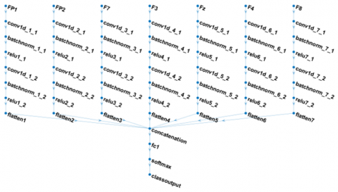
In the experimental works, we intended to investigate the channel effects on ASD detection performance. Thus, in the first experiment, only the frontal channels were considered. In other words, the FP1, FP2, F7, F3, Fz, F4 and F8 channels were used as inputs. The EEG channels FP1, FP2, F7, F3, Fz, F4, and F8 adhere to the widely recognized 10-20 system for EEG electrode placement. Each channel corresponds to a specific location on the scalp to record and analyze electrical brain activity. FP1 and FP2 are positioned at the left and right frontal pole regions, respectively. F7 and F8 are situated over the left and right frontal regions, while F3 and F4 are slightly more central within the left and right frontal areas. Fz captures activity along the midline of the forehead, providing insights into frontal region brain function. The illustration of the multi-input 1D CNN architecture for frontal channels is given in Figure 3.
Figure 3. The illustration of the multi-input 1D CNN architecture for frontal channels
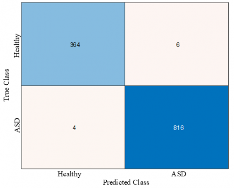
Figure 4 presents the cumulative confusion matrix derived from a 10-fold cross-validation procedure. In this matrix, the rows correspond to the true class labels of the samples, while the columns correspond to the predicted class labels, specifically distinguishing between Healthy and ASD classes. Within the context of Figure 4, it becomes evident that 6 instances belonging to the Healthy class were erroneously classified as ASD, while 4 samples from the ASD class were erroneously assigned to the Healthy category. Importantly, the application of our proposed multi-input 1D CNN model yielded a substantial number of correct classifications, accurately identifying 364 samples from the Healthy class and 816 samples from the ASD class.
Figure 4. Cumulative confusion matrix for frontal channels
Table 1 represents a comprehensive overview of performance evaluation metrics resulting from the application of multi-input 1D CNN models. The assessment focused on specific EEG channels, including FP1, FP2, F7, F3, Fz, F4, and F8, enabling a thorough evaluation of the models' capabilities. The accuracy metric reflects the models' effectiveness in correctly categorizing EEG data into Healthy and ASD classes, achieving an impressive rate of 99.16%. Sensitivity, known as the true positive rate or recall, quantifies the models' ability to identify ASD cases accurately, with a noteworthy rate of 98.38%. Specificity illustrates the models' competence in correctly identifying individuals without ASD (Healthy cases), with an outstanding rate of 99.51%. The F1-Score metric, which balances precision and recall (sensitivity), reached a significant 98.64% for these models, highlighting their ability to provide precise and reliable predictions while maintaining a robust equilibrium between precision and recall during evaluation.
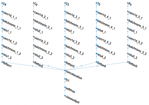
The EEG channels C4, Cz, C3, T5, and Pz correspond to specific electrode positions on the scalp, following the internationally recognized 10-20 system for EEG electrode placement. Each of these channels captures electrical brain activity from distinct regions of the scalp. C4 and C3 are situated over the right and left central areas, respectively, while Cz is located at the vertex or top center of the scalp. T5 is found on the left side, just above and behind the ear, allowing for the capture of temporal lobe activity. Finally, Pz is positioned at the top center of the parietal region. The illustration of the multi-input 1D CNN architecture for C4, Cz, C3, T5, and Pz channels is given in Figure 5.
Figure 5. The illustration of the multi-input 1D CNN architecture for frontal channels
Figure 6 displays the cumulative confusion matrix for the C4, Cz, C3, T5, and Pz channels. Within the context of Figure 6, it is evident that 12 instances from the Healthy class were erroneously classified as ASD, while eight samples from the ASD class were incorrectly assigned to the Healthy category. Importantly, our proposed multi-input 1D CNN model exhibited robust performance, accurately discerning 358 samples from the Healthy class and 812 samples from the ASD class, thereby underscoring its notable accuracy.
Table 2 presents the performance evaluation metrics for the C4, Cz, C3, T5, and Pz channels. As observed in Table 2, the achieved metrics include an accuracy of 98.32%, sensitivity of 96.76%, specificity of 99.02%, and an F1-score of 97.28%.
Figure 6. Cumulative confusion matrix for C4, Cz, C3, T5, and Pz channels
The EEG channels O1, Oz, and O2 are integral components of the international 10-20 system for EEG electrode placement, designed to capture electrical brain activity in the occipital region. O1 corresponds to the left occipital region, while O2 represents the right occipital region, with Oz positioned at the midline between them. These electrodes are strategically located to monitor and analyze brain activity associated with visual processing and other functions related to the occipital lobe, making them crucial for understanding neural processes related to vision, perception, and cognition. The illustration of the multi-input 1D CNN architecture for O1, Oz, and O2 channels is given in Figure 7.
Figure 7. The illustration of the multi-input 1D CNN architecture for O1, Oz, and O2 channels
Table 1. Performance valuation metrics obtained for multi-input 1D CNN models
|
Channels |
Accuracy (%) |
Sensitivity (%) |
Specificity (%) |
F1_Score (%) |
|
FP1, FP2, F7, F3, Fz, F4, and F8 |
99.16 |
98.38 |
99.51 |
98.64 |
Table 2. Performance valuation metrics obtained for multi-input 1D CNN models
|
Channels |
Accuracy (%) |
Sensitivity (%) |
Specificity (%) |
F1_Score (%) |
|
C4, Cz, C3, T5, and Pz |
98.32 |
96.76 |
99.02 |
97.28 |
Table 3. Performance valuation metrics obtained for multi-input 1D CNN models
|
Channels |
Accuracy (%) |
Sensitivity (%) |
Specificity (%) |
F1_Score (%) |
|
O1, Oz, and O2 |
97.65 |
95.68 |
98.54 |
96.20 |
Figure 8 indicates the cumulative confusion matrix for the O1, Oz, and O2 channels. As seen in Figure 7, 16 instances from the Healthy class were erroneously classified as ASD, while 12 samples from the ASD class were incorrectly assigned to the Healthy category. Importantly, our proposed multi-input 1D CNN model exhibited robust performance, accurately discerning 354 samples from the Healthy class and 808 samples from the ASD class, thereby underscoring its notable accuracy.
Table 3 shows the performance evaluation metrics that were obtained for O1, Oz, and O2 channels. As indicated in Table 3, the achieved performance metrics include an accuracy of 97.65%, sensitivity of 95.68%, specificity of 98.54%, and an F1-score of 96.20%.
Figure 8. Cumulative confusion matrix for O1, Oz, and O2 channels
Due to the high prevalence of ASD in children, there is a critical demand for the development of precise artificial intelligence (AI)-based tools for early diagnosis. While AI methods using electroencephalogram (EEG) data have been commonly applied in ASD diagnosis, their performance has not consistently met stringent standards. This study introduces an innovative approach that leverages a multi-input 1D CNN model. The architecture of our proposed model is designed with a sequence of one-dimensional convolutional layers, each responsible for processing signals from individual EEG channels. After the initial convolutional layer, the model incorporates batch normalization and ReLU layers. Following the first ReLU layer, an additional set of three layers, including convolutional, batch normalization, and ReLU layers, is systematically structured. The outputs from the final ReLU layers are flattened and concatenated to create an input structure for the fully connected layer. The model's architecture is completed with the inclusion of softmax and classification output layers, and the training process utilizes the 'Adam' optimization algorithm. As demonstrated in Tables 1-3, our multi-input 1D CNN model achieves impressive accuracy scores of 99.16%, 98.32%, and 97.65% across various combinations of EEG channels. It is noteworthy that recent literature has witnessed a wide array of AI-based methodologies applied to ASD diagnosis. In Table 4, we provide a comprehensive comparative summary of these approaches, with a specific focus on their utilization of EEG signals for ASD diagnosis. Hadoush et al. [23] used empirical mode decomposition-based features and neural networks for ASD detection. Pham et al. [24] used higher-order spectra bispectrum-based non-linear features and probabilistic neural networks for EEG-based ASD detection. Baygin et al. [2] used deep features and support vector classifier for EEG-based ASD detection.
As seen in Table 4, Hadoush et al. [23], Pham et al. [24], and Baygin et al. [2] obtained 97.20%, 98.70%, and 96.44% accuracy scores for their datasets. Ari et al. [7] reported three accuracy scores for various ResNet-based deep classification models. The best accuracy score that Ari et al. [7] reported was 98.88% with fine-tuning of the ResNet18 model. The proposed model produced the best accuracy score where 99.16% was produced by the proposed model.
Table 4. Comparison of the proposed approach with existing approaches.
|
Study |
Year |
Dataset |
Num. of Subjects |
Classifier |
Accuracy |
|
Hadoush et al. [23] |
2019 |
Own |
30 ASD and 30 Healthy |
ANN |
97.20% |
|
Pham et al. [24] |
2020 |
Own |
40 ASD and 37 Healthy |
PNN |
98.70% |
|
Baygin et al. [2] |
2021 |
Own |
61ASD and 61 Healthy |
SVM |
96.44% |
|
Ari et al. [7] |
2022 |
KAU |
20 ASD and 9 Healthy |
Fine-tuning of ResNet18 |
98.88% |
|
Ari et al. [7] |
2022 |
KAU |
20 ASD and 9 Healthy |
Fine-tuning of ResNet50 |
97.20% |
|
Ari et al. [7] |
2022 |
KAU |
20 ASD and 9 Healthy |
Fine-tuning of ResNet101 |
98.32% |
|
Proposed |
2023 |
KAU |
20 ASD and 9 Healthy |
Multi-input 1D CNN |
99.16% |
In conclusion, the primary objective of this manuscript was to enhance the performance of ASD detection through the utilization of EEG data. The initial dataset comprised 20 ASD cases and 9 healthy individuals, which were subsequently augmented to include 820 ASD cases and 369 healthy cases. We employed a ten-fold random partitioning approach, allocating 90% of the dataset for training and reserving the remaining 10% for testing, leading to a dataset of 1070 training samples and 119 testing samples. This process was reiterated, and average metrics were computed to ensure robustness. Our investigation was primarily centered on evaluating the influence of EEG channels on ASD detection performance. In the initial experiment, our exclusive focus was on the FP1, FP2, F7, F3, Fz, F4, and F8 channels, conforming to the widely recognized 16 EEG electrode placement system. Each of these channels corresponds to a unique scalp location responsible for the acquisition and analysis of brain activity within the frontal region. Notably, the highest accuracy score achieved was 99.16%, a result obtained through the utilization of the FP1, FP2, F7, F3, Fz, F4, and F8 channels. Subsequently, our exploration extended to the central and temporal regions of the scalp, utilizing EEG channels C4, Cz, C3, T5, and Pz, which are specialized in capturing electrical brain activity from specific regions, including the central and temporal areas. This endeavor yielded an accuracy score of 98.32%. In the final phase of our investigation, we delved into the occipital region, employing EEG channels O1, Oz, and O2, designed to capture brain activity associated with the occipital lobe, particularly in the context of visual processing and cognitive functions. The accuracy score obtained for these channels stood at 97.65%.
Our experimental findings highlighted the exceptional accuracy of the frontal electrodes, which outperformed all other experiments. Furthermore, our observations revealed a gradual reduction in accuracy scores corresponding to the decrease in the number of examined channels. A noteworthy limitation of our study pertains to the relatively small sample size, encompassing a total of 29 subjects (20 with ASD and 9 without). To address this limitation in future research endeavors, we intend to augment the validity of our model by incorporating a larger and more diverse dataset, encompassing individuals from various racial backgrounds. Additionally, our forthcoming research will extend its focus to the early detection of ASD, broadening the scope of our contributions in this critical area of study.
A potential limitation of the study lies in the exclusive reliance on EEG signals for ASD detection. While EEG provides valuable information about brain activity, it may not capture the full spectrum of complexities associated with ASD. The study focuses on specific EEG channels and employs a deep learning model tailored to this modality, potentially overlooking complementary information provided by other neuroimaging techniques like structural MRI or functional MRI. The exclusive use of EEG may limit the comprehensive understanding of ASD's neural correlates, as the disorder involves intricate interactions between various brain regions. Integrating multiple modalities could enhance the overall diagnostic accuracy and depth of insight into the neurobiological basis of ASD.
[1] Elsabbagh, M., Divan, G., Koh, Y.J., Kim, Y.S., Kauchali, S., Marcı´n, C. (2012). Global prevalence of autism and other pervasive developmental disorders. Autism Research, 5(3): 160-179. https://doi.org/10.1002/aur.239
[2] Baygin, M., Dogan, S., Tuncer, T., Barua, P.D., Faust, O., Arunkumar, N., Abdulhay, E.W., Palmer, E.E., Acharya, U.R. (2021). Automated ASD detection using hybrid deep lightweight features extracted from EEG signals. Computers in Biology and Medicine, 134: 104548. https://doi.org/10.1016/j.compbiomed.2021.104548
[3] Vicnesh, J., Wei, J.K.E., Oh, S.L., Arunkumar, N., Abdulhay, E., Ciaccio, E.J., Acharya, U.R. (2020). Autism spectrum disorder diagnostic system using HOS bispectrum with EEG signals. International Journal of Environmental Research and Public Health, 17(3): 971. https://doi.org/10.3390/ijerph17030971
[4] Bhat, S., Acharya, U.R., Adeli, H., Bairy, G.M., Adeli, A. (2014). Automated diagnosis of autism: In search of a mathematical marker. Reviews in the Neurosciences, 25(6): 851-861. https://doi.org/10.1515/revneuro-2014-0036
[5] WHO. Autism spectrum disorders, Available from: https://www.who.int/news-room/fact-sheets/detail/autism-spectrum-disorders.
[6] Oh, S.L., Jahmunah, V., Arunkumar, N., Abdulhay, E. W., Gururajan, R., Adib, N., Ciaccio, E.J., Cheong, K.H., Acharya, U.R. (2021). A novel automated autism spectrum disorder detection system. Complex & Intelligent Systems, 1-15. https://doi.org/10.1007/s40747-021-00408-8
[7] Ari, B., Sobahi, N., Alçin, Ö.F., Sengur, A., Acharya, U.R. (2022). Accurate detection of autism using Douglas-Peucker algorithm, sparse coding based feature mapping and convolutional neural network techniques with EEG signals. Computers in Biology and Medicine, 143: 105311. https://doi.org/10.1016/j.compbiomed.2022.105311
[8] Patel, M., Bhatt, H., Munshi, M., Pandya, S., Jain, S., Thakkar, P., Yoon, S. (2023). CNN-FEBAC: A framework for attention measurement of autistic individuals. Biomedical Signal Processing and Control, 105018. https://doi.org/10.1016/j.bspc.2023.105018
[9] Tawhid, M.N.A., Siuly, S., Wang, H., Whittaker, F., Wang, K., Zhang, Y. (2021). A spectrogram image based intelligent technique for automatic detection of autism spectrum disorder from EEG. Plos One, 16(6): e0253094. https://doi.org/10.1371/journal.pone.0253094
[10] Peya, Z.J., Akhand, M.A.H., Srabonee, J.F., Siddique, N. (2020). EEG based autism detection using CNN through correlation based transformation of channels' data. In 2020 IEEE Region 10 Symposium (TENSYMP), Dhaka, Bangladesh, pp. 1278-1281. https://doi.org/10.1109/TENSYMP50017.2020.9230928
[11] Xu, L., Geng, X., He, X., Li, J., Yu, J. (2019). Prediction in autism by deep learning short-time spontaneous hemodynamic fluctuations. Frontiers in Neuroscience, 13: 1120. https://doi.org/10.3389/fnins.2019.01120
[12] Loganathan, S., Geetha, C., Nazaren, A.R., Fernandez, M.H.F. (2023). Autism spectrum disorder detection and classification using chaotic optimization based Bi-GRU network: An weighted average ensemble model. Expert Systems with Applications, 230: 120613.
[13] Sharifi, Z., Momeni, H., Adabi Ardekani, H. (2023). A review of machine learning algorithms to diagnose autism using EEG signal. Soft Computing Journal. https://doi.org/10.22052/scj.2023.248522.1110
[14] Alhaddad, M.J., Kamel, M.I., Malibary, H.M., Alsaggaf, E.A., Thabit, K., Dahlwi, F., Hadi, A.A. (2012). Diagnosis autism by fisher linear discriminant analysis FLDA via EEG. International Journal of Bio-Science and Bio-Technology, 4(2): 45-54.
[15] Krizhevsky, A., Sutskever, I., Hinton, G.E. (2012). Imagenet classification with deep convolutional neural networks. Advances in Neural Information Processing Systems, 25.
[16] Simonyan, K., Zisserman, A. (2014). Very deep convolutional networks for large-scale image recognition. Computing Research Repository (CoRR), arXiv:1409.1556. https://doi.org/10.48550/arXiv.1409.1556
[17] He, K., Zhang, X., Ren, S., Sun, J. (2016). Deep residual learning for image recognition. In Proceedings of the IEEE Conference on Computer Vision and Pattern Recognition. Las Vegas, NV, USA, pp. 770-778. https://doi.org/10.1109/CVPR.2016.90
[18] Lashgari, E., Liang, D., Maoz, U. (2020). Data augmentation for deep-learning-based electroencephalography. Journal of Neuroscience Methods, 346: 108885. https://doi.org/10.1016/j.jneumeth.2020.108885
[19] Wei, Z., Zou, J., Zhang, J., Xu, J. (2019). Automatic epileptic EEG detection using convolutional neural network with improvements in time-domain. Biomedical Signal Processing and Control, 53: 101551. https://doi.org/10.1016/j.bspc.2019.04.028
[20] Omar, N. (2022). ResNet and LSTM based accurate approach for license plate detection and recognition. Traitement du Signal, 39(5): 1577-1583. https://doi.org/10.18280/ts.390514
[21] Omar, N., Sengur, A., Al-Ali, S.G.S. (2020). Cascaded deep learning-based efficient approach for license plate detection and recognition. Expert Systems with Applications, 149: 113280. http://doi.org/10.1016/j.eswa.2020.113280
[22] Tawhid, M.N.A., Siuly, S., Wang, H. (2020). Diagnosis of autism spectrum disorder from EEG using a time–frequency spectrogram image-based approach. Electronics Letters, 56(25): 1372-1375. https://doi.org/10.1049/el.2020.2646
[23] Hadoush, H., Alafeef, M., Abdulhay, E. (2019). Automated identification for autism severity level: EEG analysis using empirical mode decomposition and second order difference plot. Behavioural Brain Research, 362: 240-248. https://doi.org/10.1016/j.bbr.2019.01.018
[24] Pham, T.H., Vicnesh, J., Wei, J.K.E., Oh, S.L., Arunkumar, N., Abdulhay, E.W., Ciaccio, E.J., Acharya, U.R. (2020). Autism spectrum disorder diagnostic system using HOS bispectrum with EEG signals. International Journal of Environmental Research and Public Health, 17(3): 971. https://doi.org/10.3390/ijerph17030971