Wensi Zheng![]() | Jinsheng Cai
| Jinsheng Cai![]() | Fang Wang*
| Fang Wang*![]()
© 2024 The authors. This article is published by IIETA and is licensed under the CC BY 4.0 license (http://creativecommons.org/licenses/by/4.0/).
OPEN ACCESS
In practical engineering, the prevalence of uniform flow-induced noise poses significant challenges. Traditional models, notably Lighthill's acoustic analogy, have primarily focused on the acoustic pressure distribution, neglecting the integral role of acoustic velocity. This study introduces a novel four-dimensional (4D) acoustic wave equation model derived from the Navier-Stokes equations for fluid mechanics. This model uniquely incorporates acoustic pressure alongside three directional acoustic velocities as fundamental acoustic variables, offering a comprehensive framework for noise prediction. By integrating these variables, a 4D Ffowcs Williams-Hawkings (FW-H) equation is formulated, encapsulating the complexities of an arbitrary smooth permeable surface surrounding the noise-generating structure. Furthermore, this research innovates by establishing a time-domain integral formula for the 4D FW-H equation, incorporating a time-domain Green's function that accounts for the influence of uniform flow. Through numerical simulations involving stationary and rotating point sources within a uniformly moving medium, the efficacy of the proposed method is demonstrated. The method exhibits exceptional accuracy in capturing far-field 4D acoustic signals, aligned with analytical solutions, and reveals the characteristic Doppler effect in the acoustic fields of rotating monopole and dipole sources. A detailed investigation into the noise distribution within spatio-temporal fields under varying incident velocities, wave numbers, and propagation distances is conducted. Findings indicate a pronounced convective effect on the acoustic vector signal within a moving medium, with near-field 4D acoustic variables exhibiting nonlinear relationships with incoming flow velocity, wave number, and propagation distance, whereas far-field variables adhere to linear propagation patterns. This study diverges from conventional methodologies by considering the uniform flow's impact and devising an acoustic model capable of swiftly and accurately determining sound pressure and acoustic velocity. The developed acoustic calculation model offers valuable reference data for noise reduction and engineering structure optimization.
uniformly moving medium, flow-induced noise, vector acoustic signal, numerical simulation, Doppler effect, convective effect
Environmental pollution problems, such as noise pollution, are prevalent in transportation, industrial production, and other fields. Therefore, it is necessary to conduct a comprehensive study of the noise propagation mechanism to determine the safe distance for noise control or to implement effective noise reduction. One of the most representative research methods is the acoustic analogy proposed by Lighthill [1], which considers turbulent flow as the source of noise production, and noise propagation conforms to the linear acoustic theory. It is clear that separating the flow calculations from the noise propagation calculations can greatly improve the efficiency of the calculations. Williams and Hawkings [2] proposed the FW-H equations and elaborated on the source of noise in detail. They confirmed that the sound source of the flow can be classified into monopole, dipole, and quadrupole sources. The categorization of sound sources is a useful tool for explaining the mechanism of noise propagation, and this method offers high computational efficiency and low complexity. Farassat [3] proposed the time-domain F1 and F1A formulas in integral form based on this research idea, which is widely used in practical engineering.
All of the methods mentioned above start with the conservation form of the Navier-Stokes equations, but they can only calculate the acoustic pressure to study noise distribution. In fact, noise propagation is essentially a transformation of fluid flow energy. Sound intensity, expressed by acoustic pressure and acoustic velocity, is a more representative measure to reveal the radiation and propagation paths of noise energy. Therefore, the classical acoustic analogy method is incomplete [4]. Meanwhile, the study of acoustic velocities contributes to accurate calculations of acoustic scattering from large structures, such as the fuselage or wing [5, 6]. The acoustic scattering caused by the large boundary can significantly alter the acoustic pressure amplitude and the distribution of the incident wave [7]. To meet the impermeable boundary conditions, it is necessary to calculate the acoustic velocity [8, 9]. Therefore, using only acoustic pressure to conduct research on noise prediction is insufficient.
Research into acoustic velocities initially focused on stationary media; the acoustic pressure gradient is commonly transformed into acoustic velocity through the use of the linearized Euler equation. Therefore, most of the research work has focused on solving the pressure gradient. Farassat and Brentner [10] obtained a time-domain semi-analytical formula for the acoustic pressure gradient by directly solving the gradient of the FW-H integral equation. Lee et al. [11] then deduced the time-domain analytical formula G1A based on Farassat's research. Ghorbaniasl et al. [12] integrated the FW-H integral equation with respect to time and calculated the gradient to directly obtain the time-domain semi-analytical formulas V1 and V1A for the acoustic velocity. In contrast to the previously described method, Mao et al. [13] rederived the formulas V1 and V1A for the acoustic velocity by rearranging the fluid continuity equation and the momentum equation. He et al. [14] extracted the complete load source term from the volumetric source term and obtained the improved integral formula, which accurately calculates the acoustic velocity. The research work above only presents a fundamental method for calculating acoustic velocities in stationary media.
Aeroacoustic noise generated by airframes, wings, and rotors in a uniform flow is a well-known issue. There are typically two methods for considering the influence of a uniformly moving medium. One method involves transforming the solution for a uniform medium into the solution for a stationary medium by using the Lorentz transformation [15, 16]. However, this approach alters the surface boundary conditions and increases computational complexity [16]. Another method to obtain the integral formula of acoustic pressure is by using Green's function to consider the effect of a uniformly moving medium. Bi et al. [17] developed the time-domain acoustic pressure integral formulas for a homogeneous medium, while Ghorbaniasl et al. [18] derived the acoustic pressure integral formula in the frequency-domain for a homogeneous medium. Unfortunately, these formulas are mathematically complex and computationally intensive, making it difficult to calculate acoustic velocity in a uniform flow. The development of concise and efficient acoustic velocity formulas has become an urgent problem. Mao et al. [19] followed the FW-H equation and developed a semi-analytical formulation of acoustic velocity in a homogeneous medium. Mao's method has an issue with imprecise acoustic velocity prediction due to the omission of certain load source terms.
However, the aforementioned methods only study either acoustic pressure or acoustic velocity. A complete acoustic prediction method accurately calculating both acoustic pressure and acoustic velocity is helpful to study acoustic energy transmission and scattering effects from large structures. Kambe [20] was the first to introduce the flow field and electromagnetic field analogy to study the vortex sound theory, and the presented formulation of wave equations with entropy and acoustic velocity as integral variables is innovative. Based on Kambe's work, Dunn [4] developed a 4D Lighthill acoustic analogy for stationary media by considering the acoustic pressure and acoustic velocity in three directions as four acoustic variables. This approach resulted in a simple integral solution, which was further improved by incorporating a permeable boundary. However, Dunn's method can only predict acoustic noise in uniformly moving flow. Meanwhile, incomplete extraction of load sources may lead to numerical errors in noise calculation results.
This paper establishes a 4D acoustic analogy of a uniformly moving medium and obtains analytical formulas for the 4D acoustic vectors. Taking a fan blade or airfoil, for example, Figure 1 illustrates the propagation of acoustic vectors in a uniformly moving medium. The flow field pulsates under the influence of the incoming flow, with noise sources primarily comprising surface and volume sources. The far-field acoustic pressure and velocity can be calculated by determining the surface and volume sources. The paper is divided into four sections. A 4D acoustic analogy is presented in Section 2, and an analytical integral formula for the 4D acoustic vector is obtained by incorporating a time-domain Green's function that takes into account the effect of uniform mean flow. Section 3 validates the proposed method by carrying out numerical predictions for stationary and moving sources and comparing them with analytical solutions. The study analyzes in detail the evolution characteristics of acoustic vector signals with time and spatial location. Finally, Section 4 summarizes the entire work.
Figure 1. The mechanism of noise production and propagation in a uniform mean flow
The local flow parameters are assumed to be decomposed into two parts: the uniform incoming flow and the unsteady disturbances:
$\begin{matrix} \rho ={{\rho }_{\infty }}+{\rho }' ,& p={{p}_{\infty }}+{p}' ,& \mathbf{u}={{\mathbf{u}}_{\infty }}+\mathbf{{u}'} \\\end{matrix}$ (1)
where, ρ∞, p∞, and u∞ denote the density, pressure, and velocity of the uniform incoming flow, respectively; ρʹ, pʹ, and uʹ denote the perturbation variables.
The continuity and momentum equations satisfied by the unsteady perturbation variables can be written as:
$\frac{{{\text{D}}_{\infty }}{\rho }'}{\text{D}t}+\frac{\partial \rho {{{{u}'}}_{i}}}{\partial {{x}_{i}}}=0$ (2)
$\frac{{{\text{D}}_{\infty }}\left( \rho {{{{u}'}}_{i}} \right)}{\text{D}t}+c_{\infty }^{2}\frac{\partial {\rho }'}{\partial {{x}_{i}}}=-\frac{\partial {{T}_{ij}}}{\partial {{x}_{j}}}$ (3)
where, c∞ is the velocity of sound propagation. The Lighthill's stress tensor Tij and the material derivative D∞/Dt are given as:
${{T}_{ij}}=\rho {{{u}'}_{i}}{{{u}'}_{j}}+\left( {p}'-c_{\infty }^{2}{\rho }' \right){{\delta }_{ij}}-{{\sigma }_{ij}}$ (4)
$\frac{{{\text{D}}_{\infty }}}{\text{D}t}=\frac{\partial }{\partial t}+{{u}_{\infty i}}\frac{\partial }{\partial {{x}_{i}}}$ (5)
where, ${{\delta }_{ij}}$ and ${{\sigma }_{ij}}$ denote the Kronecker delta function and the viscous stress tensor, respectively.
Vectors E and B are introduced as:
$\mathbf{E}={{E}_{i}}=-\frac{{{\text{D}}_{\infty }}\rho {{{{u}'}}_{i}}}{\text{D}t}-c_{\infty }^{2}\frac{\partial {\rho }'}{\partial {{x}_{i}}}=\frac{\partial {{T}_{ij}}}{\partial {{x}_{j}}}$ (6)
$\mathbf{B}={{B}_{k}}={{\left( \nabla \times \rho \mathbf{{u}'} \right)}_{k}}={{\varepsilon }_{mnk}}\frac{\partial \rho {{{{u}'}}_{n}}}{\partial {{x}_{m}}}$ (7)
Combining with the above definition, the equations below automatically hold:
$\nabla \cdot \mathbf{B}=0$ (8)
$\nabla \times \mathbf{E}+\frac{{{\text{D}}_{\infty }}\mathbf{B}}{\text{D}t}=0$ (9)
2.1 The 4D Lighthill’s acoustic analogy for the uniformly moving flow
The 4D vectors and variables are firstly defined as:
${{\phi }^{\alpha }}=\left( \begin{matrix} {{\rho }'} \\ {\rho {{{{u}'}}_{1}}}/{{{c}_{\infty }}}\; \\ {\rho {{{{u}'}}_{2}}}/{{{c}_{\infty }}}\; \\ {\rho {{{{u}'}}_{3}}}/{{{c}_{\infty }}}\; \\\end{matrix} \right)=\left( \begin{matrix} {{\rho }'} \\ ------ \\ {\rho {{{{u}'}}_{i}}}/{{{c}_{\infty }}}\; \\\end{matrix} \right),\ {{X}^{\alpha }}=\left( \begin{matrix} t \\ {{x}_{1}} \\ {{x}_{2}} \\ {{x}_{3}} \\\end{matrix} \right)=\left( \begin{matrix} t \\ ---- \\ {{x}_{i}} \\\end{matrix} \right)$ (10)
The 4D differential operator and the second order tensor ηαβ are respectively represented as:
$\begin{align} & {{D}_{\alpha }}=\frac{D}{D{{X}^{\alpha }}}=\left( \begin{matrix} \frac{1}{{{c}_{\infty }}}\frac{{{\text{D}}_{\infty }}}{\text{D}t} \\ {\partial }/{\partial {{x}_{1}}}\; \\ {\partial }/{\partial {{x}_{2}}}\; \\ {\partial }/{\partial {{x}_{3}}}\; \\\end{matrix} \right)=\left( \begin{matrix} \frac{1}{{{c}_{\infty }}}\frac{{{\text{D}}_{\infty }}}{\text{D}t} \\ ------ \\ \frac{\partial }{\partial {{x}_{i}}} \\\end{matrix} \right),\ \ \ \ \ \ \ \ \ \\ & {{\eta }^{\alpha \beta }}={{\eta }_{\alpha \beta }}=\left( \begin{matrix} 1 & 0 & 0 & 0 \\ 0 & -1 & 0 & 0 \\ 0 & 0 & -1 & 0 \\ 0 & 0 & 0 & -1 \\\end{matrix} \right) \\\end{align}$ (11)
where, i=1,2,3. Xα and Dα are given as:
$\begin{align} & {{X}_{\alpha }}={{\eta }_{\alpha \beta }}{{X}^{\beta }}=\left( \begin{matrix} t \\ ---- \\ -{{x}_{i}} \\\end{matrix} \right),\ \ \ \ \ \ \\ & {{D}^{\alpha }}=\frac{D}{D{{X}_{\alpha }}}=\ {{\eta }^{\alpha \beta }}{{D}_{\beta }}=\left( \begin{matrix} \frac{1}{{{c}_{\infty }}}\frac{{{\text{D}}_{\infty }}}{\text{D}t} \\ ------ \\ -\frac{\partial }{\partial {{x}_{i}}} \\\end{matrix} \right) \\\end{align}$ (12)
where, α,β=0,1,2,3. For any three-dimensional vector e=ei and b=bi, there exists a second order antisymmetric tensor Zαβ(e,b), which has the following form:
${{Z}^{\alpha \beta }}\left( \mathbf{e},\mathbf{b} \right)=\left( \begin{matrix} 0 & -{{e}_{1}} & -{{e}_{2}} & -{{e}_{3}} \\ {{e}_{1}} & 0 & -{{b}_{3}} & {{b}_{2}} \\ {{e}_{2}} & {{b}_{3}} & 0 & -{{b}_{1}} \\ {{e}_{3}} & -{{b}_{2}} & {{b}_{1}} & 0 \\\end{matrix} \right)=\left( \begin{matrix} 0 & -{{e}_{j}} \\ {{e}_{i}} & -{{\varepsilon }_{ijk}}{{b}_{k}} \\\end{matrix} \right)$ (13)
Combining with definitions (11) and (12), the 4D convective wave operator, and the vectors E and B are given as:
$\frac{1}{c_{\infty }^{2}}\frac{\text{D}_{\infty }^{2}}{\text{D}{{t}^{2}}}-\frac{{{\partial }^{2}}}{\partial x_{i}^{2}}={{D}_{\alpha }}{{D}^{\alpha }}$ (14)
$\mathbf{E}={{E}_{i}}={{D}_{\gamma }}{{\mathbf{e}}^{\gamma }},\ \mathbf{B}={{B}_{i}}={{D}_{\gamma }}{{\mathbf{b}}^{\gamma }}$ (15)
where, the three-dimensional vectors eγ and bγ are defined as:
${{\mathbf{e}}^{\gamma }}={{\left( {{\mathbf{e}}^{\gamma }} \right)}_{i}}=\left\{ \begin{matrix} 0 & \gamma =0 \\ {{T}_{i\gamma }} & \gamma =1,2,3 \\\end{matrix} \right.,\ \ {{\mathbf{e}}^{0}}=\left( \begin{matrix} 0 \\ 0 \\ 0 \\\end{matrix} \right)\text{, }{{\mathbf{e}}^{1}}=\left( \begin{matrix} {{T}_{11}} \\ {{T}_{21}} \\ {{T}_{31}} \\\end{matrix} \right)\text{, }{{\mathbf{e}}^{2}}=\left( \begin{matrix} {{T}_{12}} \\ {{T}_{22}} \\ {{T}_{32}} \\\end{matrix} \right)\text{, }{{\mathbf{e}}^{3}}=\left( \begin{matrix} {{T}_{13}} \\ {{T}_{23}} \\ {{T}_{33}} \\\end{matrix} \right)$ (16)
$\begin{align} & {{\mathbf{b}}^{\gamma }}={{\left( {{\mathbf{b}}^{\gamma }} \right)}_{i}}=\left\{ \begin{matrix} 0 & \gamma =0 \\ {{\varepsilon }_{i\gamma k}}\rho {{{{u}'}}_{k}} & \gamma =1,2,3 \\\end{matrix} \right.,\ \ {{\mathbf{b}}^{0}}=\left( \begin{matrix} 0 \\ 0 \\ 0 \\\end{matrix} \right)\text{, } \\ & {{\mathbf{b}}^{1}}=\rho \left( \begin{matrix} 0 \\ -{{{{u}'}}_{3}} \\ {{{{u}'}}_{2}} \\\end{matrix} \right)\text{, }{{\mathbf{b}}^{2}}=\rho \left( \begin{matrix} {{{{u}'}}_{3}} \\ 0 \\ -{{{{u}'}}_{1}} \\\end{matrix} \right)\text{, }{{\mathbf{b}}^{3}}=\rho \left( \begin{matrix} -{{{{u}'}}_{2}} \\ {{{{u}'}}_{1}} \\ 0 \\\end{matrix} \right) \\\end{align}$ (17)
Similarly, Formulas (2) and (3) can be rewritten in 4D form as follows:
${{D}_{\alpha }}{{\phi }^{\alpha }}=\frac{1}{{{c}_{\infty }}}\frac{{{\text{D}}_{\infty }}{\rho }'}{\text{D}t}+\frac{\partial }{\partial {{x}_{i}}}\left( \frac{\rho {{{{u}'}}_{i}}}{{{c}_{\infty }}} \right)=0$ (18)
${{D}^{\alpha }}{{\phi }^{\beta }}-{{D}^{\beta }}{{\phi }^{\alpha }}={{D}_{\gamma }}{{V}^{\alpha \beta \gamma }}$ (19)
Here, the third-order tensor Vαβγ is expressed as:
${{V}^{\alpha \beta \gamma }}={{Z}^{\alpha \beta }}\left( \frac{{{\mathbf{e}}^{\gamma }}\ }{c_{\infty }^{2}},\frac{{{\mathbf{b}}^{\gamma }}}{{{c}_{\infty }}} \right)$ (20)
and the derivation of Formula (19) is given in the first part of the appendix.
Based on Formulas (6) and (7), the following variables are introduced:
${{q}_{0}}=\frac{1}{c_{\infty }^{2}}\nabla \cdot \mathbf{E}=\frac{1}{c_{\infty }^{2}}\frac{{{\partial }^{2}}{{T}_{ij}}}{\partial {{x}_{i}}\partial {{x}_{j}}}$ (21)
$\mathbf{q}=\frac{\nabla \times \mathbf{B}}{{{c}_{\infty }}}-\frac{1}{c_{\infty }^{3}}\frac{{{\text{D}}_{\infty }}\mathbf{E}}{\text{D}t}=\frac{{{\left( \nabla \times \left( \nabla \times \rho \mathbf{{u}'} \right) \right)}_{i}}}{{{c}_{\infty }}}-\frac{1}{c_{\infty }^{3}}\frac{{{\text{D}}_{\infty }}}{\text{D}t}\left( \frac{\partial {{T}_{ij}}}{\partial {{x}_{j}}} \right)$ (22)
By applying operator Dα to both sides of Formula (19) and combining Formulas (14) and (18), the 4D acoustic analogy for uniform mean flow is given as:
$\left( \frac{1}{c_{\infty }^{2}}\frac{\text{D}_{\infty }^{2}}{\text{D}{{t}^{2}}}-\frac{{{\partial }^{2}}}{\partial x_{i}^{2}} \right){{\phi }^{\beta }}={{D}_{\alpha }}{{D}^{\alpha }}{{\phi }^{\beta }}=\frac{{{D}^{2}}{{V}^{\alpha \beta \gamma }}}{D{{X}^{\alpha }}D{{X}^{\gamma }}}={{\mathbf{J}}^{\beta }}$ (23)
where, the source term Jβ is expressed as:
${{\mathbf{J}}^{\beta }}=\left( \begin{matrix} {{q}_{0}} \\ \mathbf{q} \\\end{matrix} \right)=\left( \frac{1}{c_{\infty }^{2}}\frac{{{\partial }^{2}}{{T}_{ij}}}{\partial {{x}_{i}}\partial {{x}_{j}}}-\frac{1}{c_{\infty }^{3}}\frac{{{\text{D}}_{\infty }}}{\text{D}t}\left( \frac{\partial {{T}_{ij}}}{\partial {{x}_{j}}} \right)+\frac{{{\left( \nabla \times \nabla \times \rho {u}' \right)}_{i}}}{{{c}_{\infty }}} \right)$. (24)
2.2 The 4D FW-H equation for the uniformly moving flow
Following the research idea of the FW-H equation, the objective of this section is to derive a generalized form of the 4D wave equation (23) in the presence of a permeable surface with moving velocity. It is assumed that the unit normal vector at the permeable surface directs from the boundary to the flow field. In combination with the relevant properties of the permeable surfaces given in the second part of the appendix, the following differential operator in vector form is defined:
${{D}_{\alpha }}f=\frac{Df}{D{{X}^{\alpha }}}={{N}_{\alpha }}\text{, }{{D}^{\alpha }}f=\frac{Df}{D{{X}_{\alpha }}}={{N}^{\alpha }}$ (25)
where, Nα and Nα are expressed as:
$\begin{align} & {{N}_{\alpha }}=\left( \begin{matrix} \frac{1}{{{c}_{\infty }}}\left( -{{v}_{j}}{{n}_{j}}+{{u}_{\infty j}}{{n}_{j}} \right) \\ {{n}_{i}} \\\end{matrix} \right), \\ & {{N}^{\alpha }}=\left( \begin{matrix} \frac{1}{{{c}_{\infty }}}\left( -{{v}_{j}}{{n}_{j}}+{{u}_{\infty j}}{{n}_{j}} \right) \\ -{{n}_{i}} \\\end{matrix} \right) \\\end{align}$ (26)
Then, DαH(f) and DαH(f) are given as:
$\begin{align} & {{D}_{\alpha }}H(f)=\delta \left( f \right)\frac{Df}{D{{X}^{\alpha }}}={{N}_{\alpha }}\delta \left( f \right),\ \ \ \ \ \\ & {{D}^{\alpha }}H(f)=\delta \left( f \right)\frac{Df}{D{{X}_{\alpha }}}={{N}^{\alpha }}\delta \left( f \right) \\\end{align}$ (27)
where, H(·) and $\delta$(·) represent the Heaviside function and the Dirac function.
By introducing the permeable surface f=0, Formula (23) can be rewritten as:
$\begin{align} & \ \ \ {{D}_{\alpha }}{{D}^{\alpha }}\left( H\left( f \right){{\phi }^{\beta }} \right)-{{D}_{\alpha }}{{D}_{\gamma }}\left( H\left( f \right){{V}^{\alpha \beta \gamma }} \right) \\ & ={{D}_{\alpha }}\left( {{D}^{\alpha }}\left( H\left( f \right){{\phi }^{\beta }} \right)-{{D}^{\beta }}\left( H\left( f \right){{\phi }^{\alpha }} \right) \right) \\ & +{{D}_{\alpha }}\left( {{D}_{\gamma }}\left( H\left( f \right){{\phi }^{\gamma }} \right){{\eta }^{\alpha \beta }}-{{D}_{\gamma }}\left( H\left( f \right){{V}^{\alpha \beta \gamma }} \right) \right) \end{align}$ (28)
and because the following equation also holds
$\begin{align} & \text{ }{{D}^{\alpha }}\left( H\left( f \right){{\phi }^{\beta }} \right)-{{D}^{\beta }}\left( H\left( f \right){{\phi }^{\alpha }} \right) \\ & +{{D}_{\gamma }}\left( H\left( f \right){{\phi }^{\gamma }} \right){{\eta }^{\alpha \beta }}-{{D}_{\gamma }}\left( H\left( f \right){{V}^{\alpha \beta \gamma }} \right) \\ & =H\left( f \right)\left( {{D}^{\alpha }}{{\phi }^{\beta }}-{{D}^{\beta }}{{\phi }^{\alpha }}+{{D}_{\gamma }}{{\phi }^{\gamma }}{{\eta }^{\alpha \beta }}-{{D}_{\gamma }}{{V}^{\alpha \beta \gamma }} \right) \\ & \text{ }+\left( {{D}^{\alpha }}H\left( f \right) \right){{\phi }^{\beta }}-\left( {{D}^{\beta }}H\left( f \right) \right){{\phi }^{\alpha }} \\ & +\left( \left( {{D}_{\gamma }}H\left( f \right) \right){{\phi }^{\gamma }} \right){{\eta }^{\alpha \beta }}-{{V}^{\alpha \beta \gamma }}{{D}_{\gamma }}\left( H\left( f \right) \right) \\\end{align}$ (29)
Combining with Formulas (20), (21) and (27), Formula (29) can be simplified as:
$\text{ }{{D}^{\alpha }}\left( H\left( f \right){{\phi }^{\beta }} \right)-{{D}^{\beta }}\left( H\left( f \right){{\phi }^{\alpha }} \right)+{{D}_{\gamma }}\left( H\left( f \right){{\phi }^{\gamma }} \right){{\eta }^{\alpha \beta }}-{{D}_{\gamma }}\left( H\left( f \right){{V}^{\alpha \beta \gamma }} \right)={{S}^{\alpha \beta }}\delta \left( f \right)$ (30)
where,
${{S}^{\alpha \beta }}={{N}^{\alpha }}{{\phi }^{\beta }}-{{N}^{\beta }}{{\phi }^{\alpha }}-{{V}^{\alpha \beta \gamma }}{{N}_{\gamma }}+{{N}_{\gamma }}{{\phi }^{\gamma }}{{\eta }^{\alpha \beta }}={{L}^{\alpha \beta }}+{{Q}^{\alpha \beta }}$ (31)
${{L}^{\alpha \beta }}={{N}^{\alpha }}{{\phi }^{\beta }}-{{N}^{\beta }}{{\phi }^{\alpha }}-{{V}^{\alpha \beta \gamma }}{{N}_{\gamma }}={{Z}^{\alpha \beta }}\left( \frac{-\mathbf{L}\ }{c_{\infty }^{2}},\mathbf{0} \right)$ (32)
${{Q}^{\alpha \beta }}={{\phi }^{\gamma }}{{N}_{\gamma }}{{\eta }^{\alpha \beta }}=\frac{Q}{{{c}_{\infty }}}{{\eta }^{\alpha \beta }}$ (33)
For convenience, the derivation of Lαβ is given in the third part of the appendix. Q and L are respectively the thickness source and the loading source proposed in FW-H equation [3]:
$Q=\left( \rho \left( {{u}_{j}}-{{v}_{j}} \right)-{{\rho }_{\infty }}\left( {{u}_{\infty j}}-{{v}_{j}} \right) \right){{n}_{j}}$ (34)
$\mathbf{L}={{L}_{i}}=\left( \rho {{{{u}'}}_{i}}\left( -{{v}_{j}}+{{u}_{j}} \right)+{p}'{{\delta }_{ij}}-{{\sigma }_{ij}} \right){{n}_{j}}$ (35)
Substituting Formula (30) into Formula (28) and reorganizing, the following equation is obtained:
$\begin{align} \left( \frac{1}{c_{\infty }^{2}}\frac{\text{D}_{\infty }^{2}}{\text{D}{{t}^{2}}}-\frac{{{\partial }^{2}}}{\partial x_{i}^{2}} \right)\left( H\left( f \right){{\phi }^{\beta }} \right) =\frac{{{D}^{2}}\left[ {{V}^{\alpha \beta \gamma }}H\left( f \right) \right]}{D{{X}^{\alpha }}D{{X}^{\gamma }}}+{{D}_{\alpha }}\left( {{S}^{\alpha \beta }}\delta \left( f \right) \right) \\\end{align}$ (36)
It is important to note that
$\begin{align} & \text{ }\frac{{{D}^{2}}\left[ {{V}^{\alpha \beta \gamma }}H\left( f \right) \right]}{D{{X}^{\alpha }}D{{X}^{\gamma }}}=\frac{{{D}^{2}}\left[ V_{1}^{\alpha \beta \gamma }H\left( f \right) \right]}{D{{X}^{\alpha }}D{{X}^{\gamma }}}\text{ }+\frac{D}{D{{X}^{\alpha }}}\left[ H\left( f \right)\frac{DV_{2}^{\alpha \beta \gamma }}{D{{X}^{\gamma }}} \right]+\frac{D}{D{{X}^{\alpha }}}\left[ V_{2}^{\alpha \beta \gamma }\frac{DH\left( f \right)}{D{{X}^{\gamma }}} \right] \\ & =\frac{{{D}^{2}}\left[ V_{1}^{\alpha \beta \gamma }H\left( f \right) \right]}{D{{X}^{\alpha }}D{{X}^{\gamma }}}+\frac{D}{D{{X}^{\alpha }}}\left( H\left( f \right)\frac{D{{V}_{2}}^{\alpha \beta \gamma }}{D{{X}^{\gamma }}} \right)\text{ }+\frac{D}{D{{X}^{\alpha }}}\left( {{Z}^{\alpha \beta }}\left( \mathbf{0},\frac{\mathbf{F}}{{{c}_{\infty }}} \right)\delta (f) \right) \\\end{align}$ (37)
where, V1αβγ, V2αβγ and F have the following form:
$\begin{align} & {{V}^{\alpha \beta \gamma }}=V_{1}^{\alpha \beta \gamma }+V_{2}^{\alpha \beta \gamma },\text{ } \\ & \begin{matrix} V_{1}^{\alpha \beta \gamma }={{Z}^{\alpha \beta }}\left( \frac{{{\mathbf{e}}^{\gamma }}\ }{c_{\infty }^{2}},\mathbf{0} \right), & V_{2}^{\alpha \beta \gamma }={{Z}^{\alpha \beta }}\left( \mathbf{0},\frac{{{\mathbf{b}}^{\gamma }}}{{{c}_{\infty }}} \right) \\\end{matrix} \\\end{align}$ (38)
$F={{N}_{\gamma }}{{\mathbf{b}}^{\gamma }}=\mathbf{n}\times \rho \mathbf{{u}'}$ (39)
Inserting Formulas (37) into Formula (36), the final form of 4D FW-H equation for the uniform mean flow is obtained as:
$\left( \frac{1}{c_{\infty }^{2}}\frac{\text{D}_{\infty }^{2}}{\text{D}{{t}^{2}}}-\frac{{{\partial }^{2}}}{\partial x_{i}^{2}} \right)\left[ H\left( f \right){{\phi }^{\beta }} \right]=\underbrace{\frac{{{D}^{2}}\left[ H\left( f \right){{V}_{1}}^{\alpha \beta \gamma } \right]}{D{{X}^{\alpha }}D{{X}^{\gamma }}}+\frac{D}{D{{X}^{\alpha }}}\left( H\left( f \right)\frac{D{{V}_{2}}^{\alpha \beta \gamma }}{D{{X}^{\gamma }}} \right)}_{\text{Volume}\ \text{source}}+\underbrace{\frac{D\left[ S_{C}^{\alpha \beta }\delta \left( f \right) \right]}{D{{X}^{\alpha }}}}_{\text{Surface}\ \text{source}}$ (40)
where, SCαβ is expressed as:
$S_{C}^{\alpha \beta }={{S}^{\alpha \beta }}+{{Z}^{\alpha \beta }}\left( \mathbf{0},\frac{\mathbf{F}}{{{c}_{\infty }}} \right)=\left( \begin{matrix} {Q}/{{{c}_{\infty }}}\; & {{{L}_{1}}}/{c_{\infty }^{2}}\; & {{{L}_{2}}}/{c_{\infty }^{2}}\; & {{{L}_{3}}}/{c_{\infty }^{2}}\; \\ -{{{L}_{1}}}/{c_{\infty }^{2}}\; & -{Q}/{{{c}_{\infty }}}\; & -{{{F}_{3}}}/{{{c}_{\infty }}}\; & {{{F}_{2}}}/{{{c}_{\infty }}}\; \\ -{{{L}_{2}}}/{c_{\infty }^{2}}\; & {{{F}_{3}}}/{{{c}_{\infty }}}\; & -{Q}/{{{c}_{\infty }}}\; & -{{{F}_{1}}}/{{{c}_{\infty }}}\; \\ -{{{L}_{3}}}/{c_{\infty }^{2}}\; & -{{{F}_{2}}}/{{{c}_{\infty }}}\; & {{{F}_{1}}}/{{{c}_{\infty }}}\; & -{Q}/{{{c}_{\infty }}}\; \\\end{matrix} \right)$ (41)
By analyzing the right side of Formula (40), it can be seen that the first two terms are volume sources, but the last term is a surface source.
2.3 The 4D time-domain FW-H integral formula for the uniform mean flow
The next key problem is to construct the integral solution of Formula (40), and the Green’s function considered the influence of uniform flow is given:
${{G}_{0}}\left( \mathbf{x},\mathbf{y},t-\tau \right)=\frac{\delta \left( g \right)}{4\pi {{R}^{*}}}$ (42)
where, symbols x and t represent the observer location and the reception time; symbols y and τ represent the sound source position and the emission time. Symbols R*, R, and g have the following form:
$\begin{align} & {{R}^{*}}={\sqrt{{{\left( r \right)}^{2}}+{{\left( \alpha \mathbf{r}\cdot {{\mathbf{M}}_{\infty }} \right)}^{2}}}}/{\alpha }\;, \\ & R={{\alpha }^{2}}\left( {{R}^{*}}-\mathbf{r}\cdot {{\mathbf{M}}_{\infty }} \right), \\ & g=t-\tau -R/{{c}_{\infty }} \\\end{align}$ (43)
r=|x-y| is the distance between source position y and observation position x, M∞=u∞/c∞ denotes Mach number of uniform mean flow, and α is the uniform flow scaling factor:
$\alpha =\frac{1}{\sqrt{1-{{\left| {{\mathbf{M}}_{\infty }} \right|}^{2}}}}$ (44)
When the main sound source is enclosed in the permeable surface, the contribution of the volume source to the sound field is ignored, and the sound field is extrapolated only by using the flow information on the permeable surface. Combined with the above Green’s function (42), the solution of equation (40) is expressed as:
${{\phi }^{\beta }}\left( \mathbf{x},t \right)=\frac{D}{D{{X}^{\alpha }}}\int_{-\infty }^{+\infty }{\int_{\mathbb{R}}{S_{C}^{\alpha \beta }\left( \mathbf{y},\tau \right)\delta \left( f \right){{G}_{0}}\text{d}{{\mathbf{y}}^{3}}\text{d}\tau }}\ =\frac{D}{D{{X}^{\alpha }}}\int_{-\infty }^{+\infty }{\int_{f=0}{S_{C}^{\alpha \beta }\left( \mathbf{y},\tau \right)\frac{\delta \left( g \right)}{4\pi {{R}^{*}}}\text{d}{{\mathbf{y}}^{2}}\text{d}\tau }}$ (45)
where,
$\begin{align} \text{ }\begin{matrix} \left| \frac{\partial g}{\partial \tau } \right|=1-{{M}_{R}} & {{M}_{R}}=\frac{{{v}_{i}}}{{{c}_{\infty }}}\frac{\partial R}{\partial {{x}_{i}}}={{M}_{i}}{{{\tilde{R}}}_{i}} \tilde{R}_{i}^{*}=\frac{\partial {{R}^{*}}}{\partial {{x}_{i}}}=\frac{{{r}_{i}}+{{\alpha }^{2}}{{M}_{\infty i}}{{r}_{k}}{{M}_{\infty k}}}{{{\alpha }^{2}}{{R}^{*}}}, & {{{\tilde{R}}}_{i}}=\frac{\partial R}{\partial {{x}_{i}}}={{\alpha }^{2}}\left( \tilde{R}_{i}^{*}-{{M}_{\infty i}} \right) \\\end{matrix} \\ & \text{ } \end{align}$ (46)
where, Mi=vi/c∞. Formula (45) is further simplified by considering the property of $\delta$(g):
$4\pi {{\phi }^{\beta }}\left( \mathbf{x},t \right)=\frac{D}{D{{X}^{\alpha }}}\int_{f=0}{{{\left[ \frac{S_{C}^{\alpha \beta }}{\left( 1-{{M}_{R}} \right){{R}^{*}}} \right]}_{ret}}\text{d}{{\mathbf{y}}^{2}}}$ (47)
$[\cdot]_{ret}$ denotes the value at retarded time. Factually, τ is the root of g=0, so that τ can be considered as the function of Xα and y based on the expression (43):
$\tau \left( {{X}^{\alpha }},\mathbf{y} \right)=t-R/{{c}_{\infty }}$ (48)
Referring to literatures [3, 21], the differential operators in Formula (47) are simplified, and the integral solution is expressed as:
$4\pi {{\phi }^{\beta }}\left( \mathbf{x},t \right)=\int_{f=0}{{{\left[ \frac{\begin{align} & {{R}^{*}}\left( 1-{{M}_{R}} \right){{D}_{\alpha }}S_{C}^{\alpha \beta } -S_{C}^{\alpha \beta }{{D}_{\alpha }}\left( {{R}^{*}}\left( 1-{{M}_{R}} \right) \right) \\\end{align}}{{{\left( {{R}^{*}}\left( 1-{{M}_{R}} \right) \right)}^{2}}} \right]}_{ret}}\text{d}{{\mathbf{y}}^{2}}}=\int_{f=0}{{{\left[ \frac{\begin{align} & {{R}^{*}}\left( 1-{{M}_{R}} \right){{K}^{\alpha \gamma }}{{\partial }_{\gamma }}S_{C}^{\alpha \beta } -S_{C}^{\alpha \beta }{{K}^{\alpha \gamma }}{{\partial }_{\gamma }}\left( {{R}^{*}}\left( 1-{{M}_{R}} \right) \right) \\\end{align}}{{{\left( {{R}^{*}}\left( 1-{{M}_{R}} \right) \right)}^{2}}} \right]}_{ret}}\text{d}{{\mathbf{y}}^{2}}}$ (49)
where, the second order tensor Kαγ and the fourth order differential operator ∂γ are:
${{K}^{\alpha \gamma }}=\left( \begin{matrix} \frac{1}{{{c}_{\infty }}} & \frac{{{u}_{\infty j}}}{{{c}_{\infty }}} \\ {{0}_{i}} & {{\delta }_{ij}} \\\end{matrix} \right)\ ,\ {{\partial }_{\gamma }}=\frac{\partial }{\partial {{X}^{\gamma }}}=\left( \begin{matrix} \frac{\partial }{\partial t} \\ \frac{\partial }{\partial {{x}_{i}}} \\\end{matrix} \right)$ (50)
And they satisfy:
${{D}_{\alpha }}={{K}^{\alpha \gamma }}{{\partial }_{\gamma }}$ (51)
The 4D vector Eγ is further defined as:
${{E}^{\gamma }}=\ {{\left[ {{\partial }_{\gamma }}\left( {{R}^{*}}\left( 1-{{M}_{R}} \right) \right) \right]}_{ret}}$ (52)
According to the law of derivatives for composite functions, the value of ∂γSCαβ at the retard time can be expressed as:
${{\left[ {{\partial }_{\gamma }}S_{C}^{\alpha \beta } \right]}_{ret}}={{\left[ \frac{\partial S_{C}^{\alpha \beta }\left( \mathbf{y},\tau \right)}{\partial \tau }\left( \frac{\partial \tau }{\partial {{X}^{\gamma }}} \right) \right]}_{ret}}={{\left[ \dot{S}_{C}^{\alpha \beta }\left( \mathbf{y},\tau \right){{C}^{\gamma }} \right]}_{ret}}$ (53)
$\begin{align} & {{E}^{\gamma }}=\ {{\left[ {{\partial }_{\gamma }}\left( {{R}^{*}}\left( 1-{{M}_{R}} \right) \right) \right]}_{ret}}\ \\ & ={{\left[ \left( 1-{{M}_{R}} \right)\left( \frac{\partial {{R}^{*}}}{\partial {{X}^{\gamma }}}+\frac{\partial {{R}^{*}}}{\partial \tau }\frac{\partial \tau }{\partial {{X}^{\gamma }}} \right) \right]}_{ret}}+{{\left[ {{R}^{*}}\left( \frac{\partial \left( 1-{{M}_{R}} \right)}{\partial {{X}^{\gamma }}}+\frac{\partial \left( 1-{{M}_{R}} \right)}{\partial \tau }\frac{\partial \tau }{\partial {{X}^{\gamma }}} \right) \right]}_{ret}} \\ & ={{\left[ \left( 1-{{M}_{R}} \right)E_{1}^{\gamma }-{{R}^{*}}E_{2}^{\gamma } \right]}_{ret}}+{{\left[ \left( \left( 1-{{M}_{R}} \right){{{\dot{R}}}^{*}}-{{R}^{*}}{{{\dot{M}}}_{R}} \right){{C}^{\gamma }} \right]}_{ret}} \\\end{align}$ (54)
where, the dot above the variable denotes the derivative with respect to the emission time, and the expressions of Cγ, E1γ and E2γ are as follows:
${{C}^{\gamma }}={{\left[ \frac{\partial \tau }{\partial {{X}^{\gamma }}} \right]}_{ret}}=\frac{1}{1-{{M}_{R}}}{{\left( \begin{matrix} 1 \\ -{{{{\tilde{R}}}_{i}}}/{{{c}_{\infty }}}\; \\\end{matrix} \right)}_{ret}}$ (55)
$E_{1}^{\gamma }=\frac{\partial {{R}^{*}}}{\partial {{X}^{\gamma }}}=\left( \begin{matrix} 0 \\ \tilde{R}_{i}^{*} \\\end{matrix} \right)$ (56)
$E_{2}^{\gamma }=\frac{\partial {{M}_{R}}}{\partial {{X}^{\gamma }}}=\frac{1}{{{R}^{*}}}\left( \begin{matrix} 0 \\ \left( {{M}_{i}}+{{\alpha }^{2}}{{M}_{j}}{{M}_{\infty j}}{{M}_{\infty i}} \right)-{{\alpha }^{2}}{{M}_{j}}\tilde{R}_{i}^{*}\tilde{R}_{j}^{*} \\\end{matrix} \right)$ (57)
The detail derivation of Formulas (55)-(57) is given in the fourth part of the appendix.
By inserting Formulas (52)-(53) into the Formula (49), the 4D time-domain FW-H integral formula for uniformly moving medium is obtained as:
$4\pi {{\phi }^{\beta }}\left( \mathbf{x},t \right)=\int_{f=0}{{{\left[ \frac{{{R}^{*}}\left( 1-{{M}_{R}} \right){{K}^{\alpha \gamma }}{{C}^{\gamma }}\dot{S}_{C}^{\alpha \beta }-{{K}^{\alpha \gamma }}{{E}^{\gamma }}S_{C}^{\alpha \beta }}{{{\left( {{R}^{*}}\left( 1-{{M}_{R}} \right) \right)}^{2}}} \right]}_{ret}}\text{d}{{\mathbf{y}}^{2}}}$ (58)
Acoustic analytical formulas are frequently validated using monopole and dipolar sources. Similarly, the acoustic radiation of monopole and dipole sources is used to verify the proposed 4D time-domain integral Eq. (58). In the Cartesian coordinate system, the uniform medium is assumed to move in the positive direction of the axis x1. The density of the uniform medium is ρ∞=1.2kg/m3, and the sound velocity is c∞=340m/s. 128 samples are evenly distributed over one period to ensure that noise signals are accurately captured. A cube with side length a=1m is chosen as the permeable surface, and 9600 square grids are uniformly distributed on the cube surface. The observation point is located in the x1-x2 plane, and the angle along counter-clockwise from the axis x1 to the direction of the observation position is assumed to be the observation angle θ. The acoustic pressure and acoustic velocity at the observation point are calculated using the 4D FW-H integral Eq. (58), where the input data on the permeable surface are calculated by the analytical solution. The derivative of the retard time is handled with a second-order central difference, and the instantaneous acoustic signals at the observation point are calculated using the advanced time algorithm [22]. As the acoustic calculations only consider the acoustic field distribution in the x1-x2 plane, the acoustic velocity along the x3 direction satisfies u3ʹ=0.
3.1 The stationary monopole source and dipole source in the uniformly moving medium
First, we consider the acoustic noise induced by the stationary monopole source located at the origin of the coordinates. The velocity potential function is given as:
$\phi \left( \mathbf{x},t \right)=\frac{A}{4\pi {{R}^{*}}}\exp \left[ \text{i}\omega \left( t-\frac{R}{{{c}_{\infty }}} \right) \right]$ (59)
where, A=1m2/s is the amplitude and $\mathrm{i}=\sqrt{-1}$. ω denotes the vibrating angular frequency of the point source, and the wavenumber is calculated with k=ω/c∞. The acoustic velocity, pressure and density are given as:
${{{u}'}_{i}}\left( \mathbf{x},t \right)=\frac{\partial \phi \left( \mathbf{x},t \right)}{\partial {{x}_{i}}},\ \ {p}'\left( \mathbf{x},t \right)=-{{\rho }_{\infty }}\frac{{{\text{D}}_{\infty }}\phi \left( \mathbf{x},t \right)}{\text{D}t},\ \ {\rho }'\left( \mathbf{x},t \right)=\frac{{p}'\left( \mathbf{x},t \right)}{c_{\infty }^{2}}$ (60)
(a) Pressure
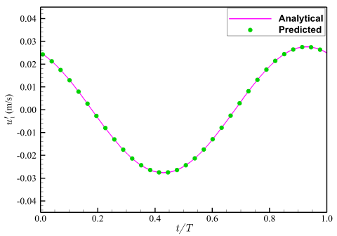
(b) Velocity u1ʹ
(c) Velocity u2ʹ
Figure 2. Time evolution of acoustic signal for monopole at θ=120̊ with the uniform flow M∞=0.6
As a validation example,the selection of wave number and Mach number does not impact the numerical predictions, as long as they align with the physical background. Based on research work in literatures [19, 21, 23], the wavenumber is chosen as k=2, and the time evolution of the acoustic vector signal at θ=120̊ for the incoming flow with M∞=0.6 is shown in Figure 2. It is demonstrated that the numerical results of the acoustic pressure and acoustic velocities are in good agreement with the analytical solutions, and they are approximately presented as single-period cosine waves. The amplitude of the acoustic pressure is much larger than that of acoustic velocities, but the amplitude of the acoustic velocity u1ʹ is larger than that of the acoustic velocity u2ʹ. That is because as the uniform medium moves from left to right along the x1 axis, the convective effect of the fluid causes the acoustic particles to move faster along the x1 direction.
Next, the reliability of the presented Formula (58) is further examined by calculating the noise distribution of the stationary dipole source. Assuming that the axis of the dipole source is aligned with the x2 axis, the velocity potential function of the stationary dipole source in a uniformly moving medium is:
$\phi \left( \mathbf{x},t \right)=\frac{\partial }{\partial {{x}_{2}}}\left\{ \frac{A}{4\pi {{R}^{*}}}\exp \left[ \text{i}\omega \left( t-\frac{R}{{{c}_{\infty }}} \right) \right] \right\}$ (61)
(a) Pressure
(b) Velocity u1ʹ
(c) Velocity u2ʹ
Figure 3. Time evolution of acoustic signals for the dipole at θ=120̊ with the uniform flow M∞=0.6
The relevant parameters for the dipole source are set up the same as those for the monopole source. Figure 3 shows the time evolution of the acoustic vector signal induced by the dipole source at the observation angle θ=120̊ for the uniformly moving medium with M∞=0.6. Numerical results for acoustic pressure and acoustic velocities are in good agreement with analytical solutions, and they are all approximately presented as sine wave distributions. Influenced by incoming flow in the horizontal direction, the amplitude variation of the dipole source is the same as that of a monopole source, and the amplitude of the acoustic velocity u1ʹ is greater than that of the acoustic velocity u2ʹ. Besides, the amplitude of the acoustic variables for the stationary dipole is approximately twice as large as that of the stationary monopole. This is because the stationary dipole source can be considered as the overlapping of two monopoles symmetrical along the x1 axis, so the noise distribution also has a cumulative effect.
3.2 The rotating monopole source in the uniformly moving medium
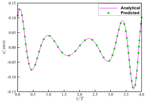
Second, the distribution of acoustic vector signals for the rotating monopole source in a uniformly moving medium is studied. Suppose the rotating monopole source is located in the x1-x2 plane, and rotates along the x3 axis with a radius r0=0.25m. The corresponding velocity potential is:
$\phi \left( \mathbf{x},t \right)=\frac{A}{4\pi {{R}^{*}}\left( 1-{{M}_{R}} \right)}\exp \left[ \text{i}\omega \left( t-\frac{R}{{{c}_{\infty }}} \right) \right]$ (62)
(a) Pressure
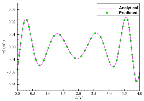
(b) Velocity u1ʹ
(c) Velocity u2ʹ
Figure 4. Time evolution of acoustic signal for rotating monopole at θ=120̊ with the uniform flow M∞=0.6
The wavenumber is chosen to be the same as that of the stationary monopole source. Figure 4 displays the time evolution of the acoustic vector signal induced by the rotating monopole at the observation angle θ=120̊ for the incoming flow with M∞=0.6, and numerical results show good agreement with analytical solutions. Unlike the stationary monopole source case, the amplitude of vector acoustic signals jumps randomly and does not behave as a sine or cosine wave with the same amplitude in each period. To further examine the directivity distribution of the acoustic field, we arrange 120 observation points uniformly on a circle with a given radius r0=12.5m in the x1-x2 plane.
(a) Pressure pʹrms
(b) Velocity uʹ1rms
(c) Velocity uʹ2rms
Figure 5. Directivities of RMS for rotating monopole with the uniform flow M∞=0.6
512 samples were continuously collected to calculate the noise distribution, and Figure 5 shows that the directivity distributions of the root mean square (RMS) for the acoustic variables are all in good agreement with those of the analytical solutions. The acoustic pressure is distributed symmetrically along the x1 axis not spatially symmetrically like a monopole. The distribution characteristics of acoustic velocities are similar to the pressure, and the acoustic velocity u1ʹ shows an asymmetric horizontal distribution with a cucurbit-shaped pattern along the x1 axis, but the acoustic velocity u2ʹ shows a standard vertical dipole distribution symmetrically along the x1 axis. The physical phenomenon described is caused by the homogeneous medium along the x1 axis. Therefore, all acoustic signals are naturally symmetrical about the horizontal axis.
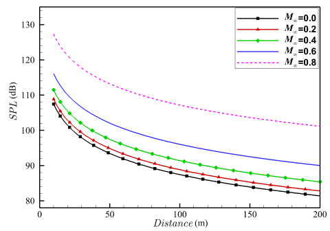
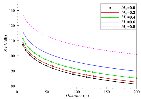
The calculations above are all based on a fixed wavenumber. However, it is important to consider the variation of acoustic signal intensity with wavenumber. Additionally, different incoming velocities can lead to dramatic variations in the acoustic field. The following discussion will focus on the impact of the incoming Mach number and wavelength on noise propagation. Along the direction of the observation angle θ=120̊, there are 200 points uniformly arranged within the interval r0$\in$[10a,200a]. The wavenumber is chosen as k=2, Figure 6 shows the sound pressure level (SPL) and the sound velocity level (SVL) of rotating monopole source with distance at different Mach numbers. The SPL and SVL were calculated with the following formulas [23]:
$\begin{align} & \text{SPL}=20{{\log }_{10}}\left( \left| {{{{p}'}}_{rms}} \right|/{{p}_{ref}} \right),\ \ \ \ \ \\ & \text{SVL}=20{{\log }_{10}}\left( \left\| {{{\mathbf{{u}'}}}_{rms}} \right\|/{{u}_{ref}} \right) \\\end{align}$ (63)
where, pref=2×10⁻⁵Pa, uref=5×10⁻⁵m/s.
(a) SPL
(b) SVL
Figure 6. Variations of SPL and SVL for rotating monopole source with different Mach number
Figure 6 demonstrates that the amplitude of SPL and SVL decays rapidly with distance. The higher the Mach number, the faster the amplitude of SPL and SVL increases at a given distance. It can be concluded that the acoustic variables of a rotating monopole source are non-linear with respect to Mach number and propagation distance, particularly for the distance r0<100a. However, the SPL and SVL at different Mach numbers are almost parallel oblique lines for the distance r0>130a. This indicates that the far-field acoustic variables are unaffected by incoming flow and decay linearly with distance, which is consistent with linear acoustic theory.
In order to specifically study the attenuation law of the noise signal, Table 1 presents the SPL amplitude of the noise signal at different incoming flow Mach numbers for wave number k=2 and r0>130a. Table 1 shows that the SPL demonstrates a linear correlation with the increase in Mach number and a decrease with propagation distance. When the propagation distance satisfies r0>130a, the SPL is affected by both the propagation distance and the Mach number. This relationship can be expressed through the following equation:
$\text{SPL}=-0.054{{r}_{0}}+92.08+\text{S}({{M}_{\infty }})$
where, S(M∞)=0.69e4.2M∞ represents the change in SPL resulting from varying incoming Mach numbers. It is important to note that as the Mach number increases, so does the value of S(M∞). There is a similar physical relationship with SVL.
Table 1. The SPL (dB) corresponding to different Mach number and propagation distance
|
M∞ r0(m) |
0.0 |
0.2 |
0.4 |
0.6 |
0.8 |
|
133.5 |
84.92 |
86.31 |
88.90 |
93.52 |
104.65 |
|
162 |
83.24 |
84.63 |
87.21 |
91.83 |
102.97 |
|
190.5 |
81.83 |
83.22 |
85.80 |
90.42 |
101.56 |
|
S(M∞) |
0.0 |
1.39 |
3.97 |
8.59 |
19.72 |
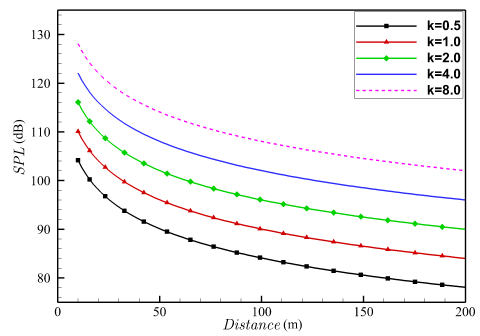
Next, we continue to study the influence of wavenumber on noise propagation. Figure 7 displays the variation of SPL and SVL with wavenumber under the incoming flow M∞=0.6. It is evident that both SPL and SVL increase uniformly with distance under the same wave number. Additionally, both SPL and SVL generally exhibit a linearly increasing trend with the wave number. Similar to the characteristics displayed in Figure 6, the SPL and SVL at different wavenumbers are almost parallel oblique lines under r0>130a. The consistency between the SPL and the SVL shown in Figures 6-7 also strongly confirms the correctness of the proposed method.
(a) SPL
(b) SVL
Figure 7. Variations of SPL and SVL for rotating monopole source under M∞=0.6 with different wavenumber
Similar to Table 1, Table 2 shows the variations of the SPL with different wave numbers and propagation distances. It can be found that the SPL increases linearly with wave number, which is also observed in Figure 7. When the propagation distance satisfies r0>130a, the SPL can also be expressed as the linear function of r0 and k:
Table 2. The SPL (dB) corresponding to different wavenumber and propagation distance
|
k r0(m) |
0.5 |
1.0 |
2.0 |
4.0 |
8.0 |
|
133.5 |
81.58 |
87.52 |
93.51 |
99.53 |
105.55 |
|
162 |
79.90 |
85.84 |
91.83 |
97.85 |
103.86 |
|
190.5 |
78.49 |
84.43 |
90.42 |
96.44 |
102.46 |
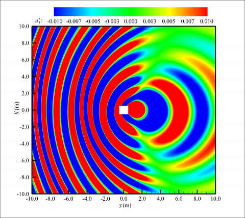
To investigate the spatial characteristic distribution of noise propagation, Figures 8-10 show the contours of the acoustic vector signal under M∞=0.6 and k=2. On one hand, the figures illustrate that the wavelength variation of three acoustic variables presents a clear Doppler effect at different times. On the other hand, the convective effect of the incoming flow also contributes to the distribution of the above vector acoustic signal. The pressure exhibits monopole characteristics, propagating outward in a circular fashion through the space.
(a) t=T/2
(b) t=T
Figure 8. Contours of the pressure at different times
(a) t=T/2
(b) t=T
Figure 9. Contours of the acoustic velocity uʹ1 at different times
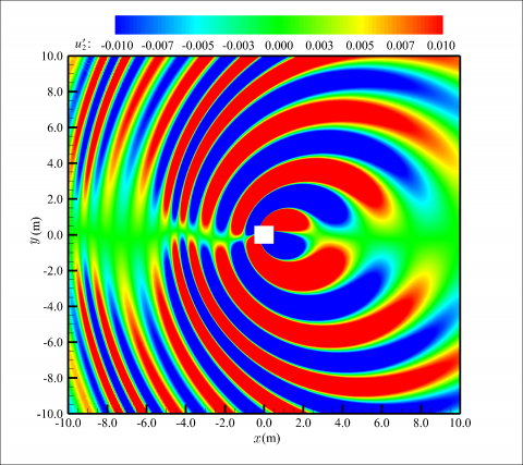
Acoustic velocities uʹ1 and uʹ2 exhibit dipole distributions. uʹ1 shows a horizontal distribution with a large value on the left and a small value on the right, while uʹ2 shows a symmetrical distribution along the horizontal axis. The characteristics shown in Figures 8-10 are the same as those in Figure 5. The biggest difference is that the amplitude of acoustic velocity uʹ2 alternates between positive and negative values along the vertical direction, which is a new phenomenon not found in previous studies.
(a) t=T/2
(b) t=T
Figure 10. Contours of the acoustic velocity uʹ2 at different times
3.3 The rotating dipole source in the uniformly moving medium
This section focuses on the noise distribution of a rotating dipole source. The velocity potential function of a moving dipole source in a uniformly moving medium is provided as
$\phi \left( \mathbf{x},t \right)=\frac{\partial }{\partial {{x}_{2}}}\left\{ \frac{A}{4\pi {{R}^{*}}\left( 1-{{M}_{R}} \right)}\exp \left[ \text{i}\omega \left( t-\frac{R}{{{c}_{\infty }}} \right) \right] \right\}$ (64)
The relevant physical parameters of the rotating dipole source are selected to be the same as those of the rotating monopole source.
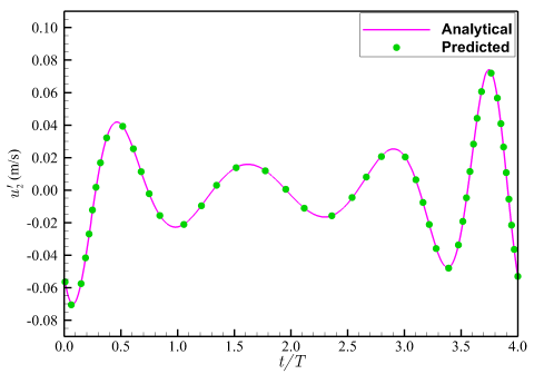
Figure 11 illustrates the distribution of acoustic variables over time at θ=120̊ and M∞=0.6. The numerical solutions for acoustic pressure and velocity in two directions are in good agreement with the analytical solutions. The amplitude of acoustic variables for the rotating dipole is almost twice as large as that of the rotating monopole shown in Figure 4.
(a) Prssure
(b) Velocity uʹ1
(c) Velocity uʹ2
Figure 11. Time evolution of acoustic variables at θ=120̊ and M∞=0.6
(a) Pressure pʹrms
(b) Velocity uʹ1rms
(b) Velocity uʹ2rms
Figure 12. Directivities of RMS for acoustic variables at M∞=0.6
Additionally, the pressure directivity, as shown in Figure 12, is also in good agreement with the analytical solution. The pressure and the acoustic velocity uʹ2 exhibit a dipole distribution, while the acoustic velocity uʹ1 exhibits a quadrupole distribution with larger values on the left and smaller values on the right. As the medium travels in the horizontal positive direction, the amplitude of the sound pressure and acoustic velocity uʹ1 on the left is significantly larger than that on the right, while the vertical acoustic velocity is almost unaffected. As a result, the acoustic velocity uʹ2 still exhibits a dipole distribution that is symmetric along the horizontal axis.
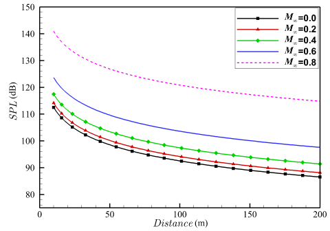
(a) SPL
(b) SVL
Figure 13. Variations of SPL and SVL with distance at different Mach numbers
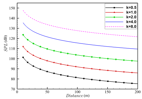
(a) SPL
(b) SVL
Figure 14. Variations of SPL and SVL with distance at different wavenumber
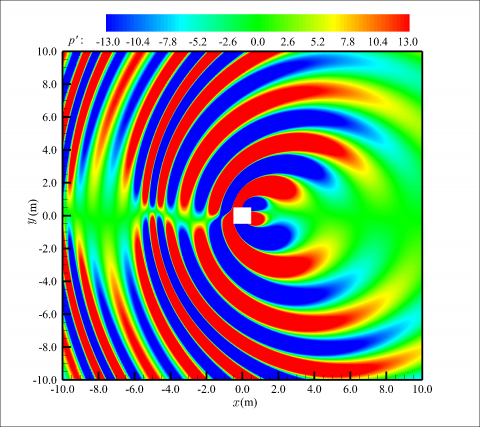
(a) t=T/2
(b) t=T
Figure 15. Contours of the sound pressure distribution at different time
(a) t=T/2
(b) t=T
Figure 16. Contours of the acoustic velocity distribution along x1 direction at different time
(a) t=T/2
(b) t=T
Figure 17. Contours of the acoustic velocity distribution along x2 direction at different time
Furthermore, this study examines the noise distribution in relation to incoming velocity and wavenumber. Similar to the rotating monopole source, there are 200 points uniformly arranged within the interval r0$\in$[10a,200a] along the direction of observation angle θ=120̊. Figure 13 displays the variations of SPL and SVL with the propagation distance for different Mach numbers at a wavenumber of k=2. Both SPL and SVL decrease rapidly with distance at the same Mach number. Furthermore, the results of SPL and SVL are completely consistent, which also confirms the accuracy of the proposed method. Figure 14 shows the variations of SPL and SVL with distance under different wave numbers at M∞=0.6. For the same propagation distance, SPL and SVL increase uniformly with the wave number. Similarly, SPL and SVL decrease linearly with propagation distance when the distance satisfies r0>130a, which accords with the linear law of far-field noise propagation.
Next, we continue to study the spatial distribution of the rotating dipole sound field at different times, selecting a wavenumber of k=2. Figures 15-17 show the spatial distributions of acoustic pressure and acoustic velocity at the incoming Mach number M∞=0.6. As can be seen from these figures, the sound field exhibits an obvious Doppler effect at different moments. In particular, Figure 15 shows that the acoustic pressure distribution exhibits dipole characteristics, while Figure 16 shows the quadrupole characteristics in acoustic velocity uʹ1, and Figure 17 shows the dipole characteristics in acoustic velocity uʹ2. At moments T/2 and T, both the acoustic pressure and the acoustic velocities spatially simultaneously exhibit alternating negative and positive values. Meanwhile, the convection effect of the medium also has a large impact on the sound field, the waves in the left propagation region appear to be compressed, while those on the right appear to be expanding. This is in contrast to the noise distribution of the monopole source discussed in Section 3.2.
When calculating acoustic energy, it is important to consider the completeness of the acoustic variables and the influence of the incoming flow. In this paper, the Navier-Stokes equations of fluid mechanics are used to reorganize the continuity and momentum equations into 4D convective wave equations with variables of acoustic pressure and acoustic velocity. Then, a time-domain 4D FW-H integral formula is suggested for uniformly mean flow along with a permeable boundary. This can solve the acoustic pressure and acoustic velocity at the same time, taking into account the convective effect. The main conclusions are as follows:
(1) The numerical solutions for acoustic pressure and acoustic velocity obtained by the proposed method are in good agreement with the analytical solutions for monopole sources and dipole sources. This fully demonstrates that the proposed method can accurately capture the characteristic distributions and propagation laws of acoustic pressure and velocity in a uniform mean flow. The 4D FW-H integral formula can be applied to calculate vector acoustic noise for moving sources and noise reception problems for moving observers.
The method proposed in this study uses the permeable surface as the sound source extraction surface, which is a practical and straightforward approach.
(2) The Doppler effect and convective effect of the rotating point source changes the linear and uniform distribution of the acoustic field, especially in the near-field region. As shown in Figures 6-7, SPL and SVL decrease as the acoustic propagation distance increases at different incoming Mach numbers. There is a sharp decrease in the near-field region, followed by a linear propagation pattern in the far-field region. The oscillation frequency of the point source, the wavenumber, has a similar impact on acoustic propagation as the incoming Mach number. However, the acoustic signals are amplified linearly and uniformly with an increase in wavenumber and more rapidly with an increase in Mach number. As shown in Tables 1-2, when the distance satisfies r0>130a, one quantitative relationship exists between SPL and Mach number M∞ as SPL=-0.054r0+92.08+0.69e4.2M∞, another quantitative relationship exists between SPL and wavenumber k as SPL=-0.054r0+84.7+8.66lnk. This indicates that the magnitude of the uniform mean flow has a significant impact on both the intensity and distribution of the acoustic signals.
(3) Unlike earlier studies, the 4D FW-H formula can directly figure out the acoustic pressure and velocity by using smooth permeable surfaces around the object. This is a general model that can be used for any complex structure. Therefore, the distribution and transmission mechanisms of acoustic intensity expressed with acoustic pressure and acoustic velocity are easy to study. However, in practical engineering applications, if the selected permeable surface cannot contain all the nonlinear regions, the vortex wave perturbation on the permeable integral surface will be input as real acoustic source data, which will generate pseudoacoustic phenomena and result in inaccurate sound field calculations. In the future, researchers will try to come up with a similar pseudoacoustic suppression method using the 4D acoustic analogy described in this paper. For example, they could look at how to figure out the contribution of quadrupole sources outside permeable surfaces with extra surface sources, how to break down acoustic and vortex waves, and so on. Additionally, research will be conducted on predicting aerodynamic noise for practical problems.
The research was supported by the Natural Science Foundation of Ningxia (Grant No.: 2021AAC03209 and 2023AAC03299), and the research project of the National Key Laboratory of Science and Technology on Aerodynamic Design and Research (Grant No.: 614220120030115).
1. The derivation of 4D momentum equations
Combined with the definitions of Eqs. (10) and (12)
${{D}^{\alpha }}{{\phi }^{\beta }}-{{D}^{\beta }}{{\phi }^{\alpha }}=\left( \begin{matrix} 0 & \frac{1}{c_{\infty }^{2}}\frac{{{\text{D}}_{\infty }}\rho {{{{u}'}}_{j}}}{\text{D}t}+\frac{\partial {\rho }'}{\partial {{x}_{j}}} \\ -\frac{\partial {\rho }'}{\partial {{x}_{i}}}-\frac{1}{c_{\infty }^{2}}\frac{{{\text{D}}_{\infty }}\rho {{{{u}'}}_{i}}}{\text{D}t} & -\frac{1}{{{c}_{\infty }}}\frac{\partial \rho {{{{u}'}}_{j}}}{\partial {{x}_{i}}}+\frac{1}{{{c}_{\infty }}}\frac{\partial \rho {{{{u}'}}_{i}}}{\partial {{x}_{j}}} \\\end{matrix} \right)$ (A1)
Because
$\frac{\partial \rho {{{{u}'}}_{i}}}{\partial {{x}_{j}}}-\frac{\partial \rho {{{{u}'}}_{j}}}{\partial {{x}_{i}}}=({{\delta }_{in}}{{\delta }_{jm}}-{{\delta }_{im}}{{\delta }_{jn}})\frac{\partial \rho {{{{u}'}}_{n}}}{\partial {{x}_{m}}}=-{{\varepsilon }_{ijk}}{{\varepsilon }_{kmn}}\frac{\partial \rho {{{{u}'}}_{n}}}{\partial {{x}_{m}}}=-{{\varepsilon }_{ijk}}{{B}_{k}}$ (A2)
Based on the Eq. (A2), the Eq. (A1) is further simplified
${{D}^{\alpha }}{{\phi }^{\beta }}-{{D}^{\beta }}{{\phi }^{\alpha }}=\left( \begin{matrix} 0 & -\frac{{{E}_{j}}}{c_{\infty }^{2}} \\ \frac{{{E}_{i}}}{c_{\infty }^{2}} & -\frac{{{\varepsilon }_{ijk}}{{B}_{k}}}{{{c}_{\infty }}} \\\end{matrix} \right)={{Z}^{\alpha \beta }}\left( \frac{\mathbf{E}}{c_{\infty }^{2}},\frac{B}{{{c}_{\infty }}} \right)$ (A3)
Applying the Eq. (15) to the Eq. (A3), it is further obtained
${{D}^{\alpha }}{{\phi }^{\beta }}-{{D}^{\beta }}{{\phi }^{\alpha }}={{Z}^{\alpha \beta }}\left( \frac{{{D}_{\gamma }}{{\mathbf{e}}^{\gamma }}\ }{c_{\infty }^{2}},\frac{{{D}_{\gamma }}{{\mathbf{b}}^{\gamma }}}{{{c}_{\infty }}} \right)={{D}_{\gamma }}{{V}^{\alpha \beta \gamma }}$ (A4)
where the third order tensor Vαβγ is defined as
${{V}^{\alpha \beta \gamma }}={{Z}^{\alpha \beta }}\left( \frac{{{\mathbf{e}}^{\gamma }}\ }{c_{\infty }^{2}},\frac{{{\mathbf{b}}^{\gamma }}}{{{c}_{\infty }}} \right)$ (A5)
2. Relevant properties of permeable surface $f=0$
As given in the literature [3], the inner and outer regions of the permeable surface are defined respectively as f<0 and f>0. Let the unit outer normal vector of the permeable surface be $n=\nabla f$, satisfying the following relation
$\frac{\partial f}{\partial t}=-{{v}_{j}}{{n}_{j}}$ (A6)
H(·) is the Heaviside step function
$H\left( f \right)=\left\{ \begin{matrix} 0, & f<0 \\ 1, & f>0 \\\end{matrix} \right.$ (A7)
and satisfy
$\frac{\partial H\left( f \right)}{\partial t}+{{v}_{j}}\frac{\partial H\left( f \right)}{\partial {{x}_{j}}}=0$ (A8)
According to the law of derivatives for composite functions
$\frac{\partial H\left( f \right)}{\partial {{x}_{j}}}=\frac{\partial f}{\partial {{x}_{j}}}\frac{\partial H\left( f \right)}{\partial f}={{n}_{j}}\delta \left( f \right)$ (A9)
where, δ(·) is the Dirac function. Using Eqs. (A8) and (A9) yields
$\frac{\partial H\left( f \right)}{\partial t}=-{{v}_{j}}{{n}_{j}}\delta \left( f \right)$ (A10)
3. The specific form of Lαβ
${{L}^{\alpha \beta }}={{N}^{\alpha }}{{\phi }^{\beta }}-{{N}^{\beta }}{{\phi }^{\alpha }}-{{V}^{\alpha \beta \gamma }}{{N}_{\gamma }}={{Z}^{\alpha \beta }}\left( \frac{\ {{\mathbf{A}}_{1}}}{c_{\infty }^{2}},\frac{\mathbf{F}}{{{c}_{\infty }}} \right)-{{Z}^{\alpha \beta }}\left( \frac{{{\mathbf{A}}_{2}}\ }{c_{\infty }^{2}},\frac{\mathbf{F}}{{{c}_{\infty }}} \right)\ ={{Z}^{\alpha \beta }}\left( -\frac{\ \mathbf{L}}{c_{\infty }^{2}},\mathbf{0} \right)$. (A11)
Here, the three dimensional vectors A1, A2 and L defined as
${{\mathbf{A}}_{1}}={{\left( {{\mathbf{A}}_{1}} \right)}_{i}}=-{\rho }'{{n}_{i}}c_{\infty }^{2}-\rho {{{u}'}_{i}}\left( -{{v}_{n}}+{{u}_{\infty n}} \right)$ (A12)
${{\mathbf{A}}_{2}}={{N}_{\gamma }}{{\mathbf{e}}^{\gamma }}={{\left( {{\mathbf{A}}_{2}} \right)}_{i}}={{n}_{j}}{{T}_{ij}}$ (A13)
$\mathbf{L}={{\mathbf{A}}_{2}}-{{\mathbf{A}}_{1}}=\left( \rho {{{{u}'}}_{i}}\left( -{{v}_{j}}+{{u}_{j}} \right)+{p}'{{\delta }_{ij}}-{{\sigma }_{ij}} \right){{n}_{j}}$ (A14)
4. The derivation of Cγ, E1γ and E2γ
For the term Cγ
${{C}^{\gamma }}={{\left[ \frac{\partial \tau }{\partial {{X}^{\gamma }}} \right]}_{ret}}={{\left( \begin{matrix} \frac{\partial \tau }{\partial t} \\ \frac{\partial \tau }{\partial {{x}_{i}}} \\\end{matrix} \right)}_{ret}}$ (A15)
The retarded time τ can be considered as the function of the variables Xα and y, and τ(Xα,y) satisfies
$0=g=t-\tau -{R}/{{{c}_{\infty }}}\;$ (A16)
Find derivations on the Eq. (16) with respect to t
$0=1-\frac{\partial \tau }{\partial t}-\frac{1}{{{c}_{\infty }}}\frac{\partial R}{\partial \tau }\frac{\partial \tau }{\partial t}=1+\left( -1+{{M}_{R}} \right)\frac{\partial \tau }{\partial t}$ (A17)
It can be expressed as
$\frac{\partial \tau }{\partial t}=\frac{1}{1-{{M}_{R}}}$ (A18)
Taking the spatial derivative of Eq. (A16) yields
$0=-\frac{\partial \tau }{\partial {{x}_{i}}}-\frac{1}{{{c}_{\infty }}}\left( \frac{\partial R}{\partial {{x}_{i}}}+\frac{\partial R}{\partial \tau }\frac{\partial \tau }{\partial {{x}_{i}}} \right)=-\frac{1}{{{c}_{\infty }}}{{\tilde{R}}_{i}}+\left( -1+{{M}_{R}} \right)\frac{\partial \tau }{\partial {{x}_{i}}}$ (A19)
It is further expressed as
$\frac{\partial \tau }{\partial {{x}_{i}}}=\frac{-{{{\tilde{R}}}_{i}}}{{{c}_{\infty }}\left( 1-{{M}_{R}} \right)}$ (A20)
Substituting Eqs. (A18) and (A20) into the Eq. (A15)
${{C}^{\gamma }}={{\left( \frac{\partial \tau }{\partial {{X}^{\gamma }}} \right)}_{ret}}=\frac{1}{1-{{M}_{R}}}{{\left( \begin{matrix} 1 \\ -{{{{\tilde{R}}}_{i}}}/{{{c}_{\infty }}}\; \\\end{matrix} \right)}_{ret}}$ (A21)
The term E1γ satisfies
$E_{1}^{\gamma }={{\left[ \frac{\partial {{R}^{*}}}{\partial {{X}^{\gamma }}} \right]}_{ret}}={{\left( \begin{matrix} \frac{\partial {{R}^{*}}}{\partial t} \\ \frac{\partial {{R}^{*}}}{\partial {{x}_{i}}} \\\end{matrix} \right)}_{ret}}=\left( \begin{matrix} 0 \\ \tilde{R}_{i}^{*} \\\end{matrix} \right)$ (A22)
For the term E2γ
$E_{2}^{\gamma }={{\left[ \frac{\partial {{M}_{R}}}{\partial {{X}^{\gamma }}} \right]}_{ret}}={{\left( \begin{matrix} \frac{\partial {{M}_{R}}}{\partial t} \\ \frac{\partial {{M}_{R}}}{\partial {{x}_{i}}} \\\end{matrix} \right)}_{ret}}={{\left( \begin{matrix} 0 \\ \frac{\partial {{M}_{R}}}{\partial {{x}_{i}}} \\\end{matrix} \right)}_{ret}}$ (A23)
Using the definition of MR
$\frac{\partial {{M}_{R}}}{\partial {{x}_{i}}}=\frac{\partial \left( {{{\tilde{R}}}_{j}}{{M}_{j}} \right)}{\partial {{x}_{i}}}={{\alpha }^{2}}{{M}_{j}}\frac{\partial \tilde{R}_{j}^{*}}{\partial {{x}_{i}}}$ (A24)
Among them, the expression for ${\partial \tilde{R}_{j}^{*}}/{\partial {{x}_{i}}}\;$ is
$\frac{\partial \tilde{R}_{j}^{*}}{\partial {{x}_{i}}}=\frac{1}{{{\alpha }^{2}}}\left\{ \frac{1}{{{R}^{*}}}\left( {{\delta }_{ij}}+{{\alpha }^{2}}{{M}_{\infty j}}{{M}_{\infty i}} \right)-\frac{{{\alpha }^{2}}\tilde{R}_{i}^{*}\tilde{R}_{j}^{*}}{{{R}^{*}}} \right\}$ (A25)
Combining Eqs. (A24) and (A25), the Eq. (A23) is reduced to
$E_{2}^{\gamma }=\frac{1}{{{R}^{*}}}\left( \begin{matrix} 0 \\ {{M}_{i}}+{{\alpha }^{2}}{{M}_{j}}{{M}_{\infty j}}{{M}_{\infty i}}-{{\alpha }^{2}}{{M}_{j}}\tilde{R}_{i}^{*}\tilde{R}_{j}^{*} \\\end{matrix} \right)$ (A26)
[1] Lighthill, M.J. (1952). On sound generated aerodynamically. I. General Theory. Proceedings of the Royal Society of London, Series A: Mathematical and Physical Sciences, 211(1107): 564-587.
[2] Williams, J.F., Hawkings, D.L. (1969). Sound generation by turbulence and surfaces in arbitrary motion. Philosophical Transactions for the Royal Society of London. Series A, Mathematical and Physical Sciences, 264(1151): 321-342.
[3] Farassat F. (2007). Derivation of Formulations 1 and 1A of Farassat. NASA Technical Report TM-2007-214853.
[4] Dunn, M.H. (2019). The Acoustic analogy in four dimensions. International Journal of Aeroacoustics, 18(8): 711-751.
[5] Roger, M., Moreau, S., Kucukcoskun, K. (2016). On sound scattering by rigid edges and wedges in a flow, with applications to high-lift device aeroacoustics. Journal of Sound and Vibration, 362: 252-275. https://doi.org/10.1016/j.jsv.2015.10.004
[6] Gaffney, J., McAlpine, A., Kingan, M.J. (2018). A theoretical model of fuselage pressure levels due to fan tones radiated from the intake of an installed turbofan aero-engine. The Journal of the Acoustical Society of America, 143(6): 3394-3405. https://doi.org/10.1121/1.5038263
[7] Crighton, D.G., Leppington, F.G. (1971). On the scattering of aerodynamic noise. Journal of Fluid Mechanics, 46(3): 577-597. https://doi.org/10.1017/S0022112071000715
[8] Lee, S., Brentner, K.S., Morris, P.J. (2012). Time-domain approach for acoustic scattering of rotorcraft noise. Journal of the American Helicopter Society, 57(4): 1-12. https://doi.org/10.4050/JAHS.57.042001
[9] Lee, S., Brentner, K.S., Morris, P.J. (2010). Acoustic scattering in the time domain using an equivalent source method. AIAA Journal, 48(12): 2772-2780. https://doi.org/10.2514/1.45132
[10] Farassat, F., Brentner, K.S. (2005). The derivation of the gradient of the acoustic pressure on a moving surface for application to the fast scattering code (FSC) (No. NASA/TM-2005-213777).
[11] Lee, S., Brentner, K.S., Farassat, F., Morris, P.J. (2009). Analytic formulation and numerical implementation of an acoustic pressure gradient prediction. Journal of Sound and Vibration, 319(3-5): 1200-1221. https://doi.org/10.1016/j.jsv.2008.06.028
[12] Ghorbaniasl, G., Carley, M., Lacor, C. (2013). Acoustic velocity formulation for sources in arbitrary motion. AIAA Journal, 51(3): 632-642. https://doi.org/10.2514/1.J051958
[13] Mao, Y., Tang, H., Xu, C. (2016). Vector wave equation of aeroacoustics and acoustic velocity formulations for quadrupole source. AIAA Journal, 54(6): 1922-1931. https://doi.org/10.2514/1.J054687
[14] He, J., Xue, S., Liu, Q., Yang, D., Wang, L. (2023). Acoustic velocity analogy formulation for sources in quiescent medium. Proceedings of the Institution of Mechanical Engineers, Part G: Journal of Aerospace Engineering, 237(13): 3018-3031. https://doi.org/10.1177/09544100231174332
[15] Hu, F.Q., Pizzo, M.E., Nark, D.M. (2019). On the use of a Prandtl-Glauert-Lorentz transformation for acoustic scattering by rigid bodies with a uniform flow. Journal of Sound and Vibration, 443: 198-211. https://doi.org/10.1016/j.jsv.2018.11.043
[16] Wang, Z.H., Rienstra, S.W., Bi, C.X., Koren, B. (2020). An accurate and efficient computational method for time-domain aeroacoustic scattering. Journal of Computational Physics, 412: 109442. https://doi.org/10.1016/j.jcp.2020.109442
[17] Bi, C.X., Wang, Z.H., Zhang, X.Z. (2017). Analytic time-domain formulation for acoustic pressure gradient prediction in a moving medium. AIAA Journal, 55(8): 2607-2616. https://doi.org/10.2514/1.J055630
[18] Ghorbaniasl, G., Huang, Z., Siozos-Rousoulis, L., Lacor, C. (2015). Analytical acoustic pressure gradient prediction for moving medium problems. Proceedings of the Royal Society A: Mathematical, Physical and Engineering Sciences, 471(2184): 20150342. https://doi.org/10.1098/rspa.2015.0342
[19] Mao, Y., Hu, Z., Xu, C., Ghorbaniasl, G. (2018). Vector aeroacoustics for uniform mean flow: Acoustic velocity and vortical velocity. AIAA Journal, 56(7): 2782-2793. https://doi.org/10.2514/1.J056852
[20] Kambe, T. (2010). A new formulation of equations of compressible fluids by analogy with Maxwell's equations. Fluid Dynamics Research, 42(5): 055502. https://doi.org/10.1088/0169-5983/42/5/055502
[21] Najafi-Yazdi, A., Brès, G.A., Mongeau, L. (2011). An acoustic analogy formulation for moving sources in uniformly moving media. Proceedings of the Royal Society A: Mathematical, Physical and Engineering Sciences, 467(2125): 144-165. https://doi.org/10.1098/rspa.2010.0172
[22] Casalino, D. (2003). An advanced time approach for acoustic analogy predictions. Journal of Sound and Vibration, 261(4): 583-612. https://doi.org/10.1016/S0022-460X(02)00986-0
[23] Xu, C., Mao, Y., Hu, Z., Ghorbaniasl, G. (2018). Vector aeroacoustics for a uniform mean flow: Acoustic intensity and acoustic power. AIAA Journal, 56(7): 2794-2805.