Suganya Asokan![]() | Aarthy Seshadri*
| Aarthy Seshadri*![]()
© 2023 IIETA. This article is published by IIETA and is licensed under the CC BY 4.0 license (http://creativecommons.org/licenses/by/4.0/).
OPEN ACCESS
The precise diagnosis of neurodegenerative disorders, notably Parkinson's disease (PD) and Alzheimer's disease (AD), presents a formidable challenge, often necessitating several years for definitive determination. Given the increasing prevalence of PD and AD in aging populations of affluent nations, there is an urgent need for advanced technology and more precise diagnostic methodologies, particularly for early disease stages. In recent years, segmentation has seen a surge in application for processing Magnetic Resonance (MR) brain data, emerging as a valuable and indispensable tool. To capture comprehensive images of the brain for the diagnosis and classification of these neurodegenerative disorders, Magnetic Resonance Imaging (MRI) is employed. However, early detection and classification of PD and AD utilizing MRI datasets pose significant complexities. Owing to the inherent subjectivity of human observation, automated segmentation of MRI images has become a crucial asset for healthcare professionals. The primary focus of this study is to devise an effective image segmentation approach and classification techniques for the detection and categorization of AD and PD. Initially, Hierarchical Spatial Feature-CNN is employed to segment abnormal traces of PD and AD in MRIs. Subsequently, the Gradient-weighted Class Activation Mapping (Grad-CAM) method is used for disease classification. In Grad-CAM, each neuron is assigned prioritization weights based on their contribution to the classification of interest, using gradient information flowing into the final convolutional layer of the Convolutional Neural Network (CNN). Thus, the combination of Grad-CAM with CNN is applied to address the classification challenges inherent in PD and AD. Extensive experiments were conducted on the proposed model, resulting in a classification accuracy exceeding 98.17%. In addition, the proposed integration of Grad-CAM with CNN outperformed existing state-of-the-art approaches across all performance measures. This study underscores the potential of the proposed model in enhancing the diagnostic process for neurodegenerative disorders, offering promise for more efficient and accurate detection and classification of PD and AD.
accuracy, classification, segmentation, Alzheimer’s, Parkinson’s, features, Magnetic Resonance Imaging, Convolutional Neural Network, Grad-CAM
Globally, countless individuals are grappling with neurodegenerative disorders, notably Parkinson's disease (PD) and Alzheimer's disease (AD). AD is marked by an insidious cognitive decline, encompassing learning difficulties [1], compromised cognition, memory deficits, and impaired executive thinking [2]. Furthermore, non-motor symptoms such as disorientation, anxiety, and parasympathetic dysfunctions may also manifest [3]. PD, on the other hand, is characterized by a deterioration in cognitive abilities, a loss of muscle control, and the eventual induction of apoptosis. Both PD and AD exhibit a similar pattern of gradual symptom onset, leading to severe brain damage over the extended prodromal phase. The challenge lies in discerning whether the brain damage is attributable to Alzheimer's disease or Parkinson's disease, which complicates the process of accurately pinpointing the disease condition during the diagnosis.
Image segmentation enables the separation of the foreground in medical scans (ranging from MRIs to CT scans) from the pixel intensities representing structures and abnormalities [4]. Image segmentation [5] refers to the process of partitioning a digital image into smaller segments based on shared visual characteristics such as brightness, structure, texture, or color. This procedure simplifies the task of extracting features like structure, color, and shape from digital images [6] by grouping pixels into clusters based on the similarity of pixel intensity levels in the original image. Consequently, images are divided into clusters of pixels sharing common characteristics. It is imperative that these groups do not overlap and that the neighboring subgroups are diverse and distinct [7]. Image segmentation functions by classifying all pixels such that adjacent pixels share common labeling [8].
In the diagnosis and treatment of these debilitating diseases, clinical visual segmentation has proven to be an indispensable tool. A variety of imaging techniques, including MRI, PET, thermography, CT, X-ray-CT, OCT, US, TI, among others, are utilized to collect clinical data. The MRI technique, a non-invasive diagnostic modality, is capable of capturing highly detailed three-dimensional anatomical images [9-11]. Magnetic Resonance Imaging facilitates the precise analysis of neurodegenerative disorders, making MRI-based image feeds the focus of this proposed research endeavor.
Volumetric assessment of structural scans has risen to prominence as the principal screening indicator in large-scale prospective studies and the testing of treatments for sporadic symptomatic dementia, as endorsed by Western medicine standards [12,13]. This approach is also used in the case of pre-symptomatic biological brain disorders [14]. Prognosis for AD sufferers ranges from 8-15 years from the onset of symptoms. Figure 1(a) provides a visual representation of the prevalence of AD.
Figure 1. (a) Prevalence of AD (b) Prevalence of PD
Following AD, Parkinson's Disease (PD) stands as perhaps the most prevalent form of neurodegeneration. Diagnostically, PD is characterized by the gradual apoptosis of neurons in the substantia nigra region and other areas, coupled with the presence of ubiquitinated grey matter within the neurons. Moreover, individuals with PD frequently struggle with emotional management, particularly anxiety and depression. Figure 1(b) offers a visual representation of the prevalence of PD.
While the impacts of these diseases are readily distinguishable, the task of isolating the affected area from various neuroimaging techniques, particularly MRIs, presents a significant challenge. The segmentation process has increasingly become complex and demanding. Primary causes of categorization issues include fixed magnetic permeability, RF penetration, and subjects' motion during image acquisition [15, 16]. This study, therefore, zeroes in on the specific challenges posed by the segmentation and categorization of these diseases using standard brain MRI datasets.
Numerous scholarly investigations have delved into the practice of image segmentation in brain MRIs. As such, this section presents a thorough research analysis of the diverse methods proposed for accurately segmenting brain MRI. The Multiple Atlas-based visual Segmentation method, which involves the creation of numerous atlases [17], has been found to yield the best segmentation outcomes. The effectiveness of these techniques hinges on an accurate template-to-image spatial analysis [18].
A group-wise registration utilizing a tree-based approach is proposed to match both the atlas and the target image simultaneously. In the intermediate step of the multi-group segmentation technique, each image's atlas is combined with the most consistently segmented target images [19]. Occasionally, multiple branches are taken from the root of the tree. Employing Kruskal's method, researchers have calculated the minimal tree structure to identify the smallest possible set of connected nodes. To minimize labeling inaccuracies, a fusion of label fusion with multi-atlas segmentation techniques has been implemented using a voting system. The joint probability of multiple atlases is used to precisely characterize the mapping [20].
Unsupervised methods, unlike those used in cluster-based segmentation approaches, do not require a data source to learn from. The BCFCM method addresses the estimation and restoration in brain MRI for approximating, segmenting, and classifying in a single step [21]. The FCM method is made more effective by incorporating regional context. Variations include bilateral BCFCM, BCFCM, adaptive non-local FCM, multi-scale, and multi-block FCM [22], rough-set FCM, simplified rough-set FCM [23], improved FCM [24], simplified kernel FCM, and others.
In the structure-based model used in the SOM-based segmentation approach, descriptors (features) were developed to categorize preferred pixel regions in brain MRIs. To prevent any single feature representation from becoming overly dominant, position and aspect invariants were extracted from the MRI's 2D sequencing and then normalized before being used to construct the feature vector [25]. When selecting the best-matching units, loss metrics are considered for the quality of fit. An Expanding Hierarchical-SOM framework was developed by researchers for image classification using calculated selected features [26].
The fundamental premise of the contour-based segmentation approach is that distinct tissues can be differentiated by tracing their perimeters. Segmentation techniques that rely on deformable models are widely used to dissect medical imagery [27]. Benefits of deformable approaches include the ability to generate localized curves and surfaces from images and the ease of incorporating smoothing constraints; these models also exhibit resilience to noise and deceptive features. However, the deformable approach also carries the downside of subpar fitting to concave boundaries.
The variational thresholding method has been employed to establish a framework for region-based Active Contour Models (ACM). The contour is set into motion by summing all energy values [28]. Now, diverse sections of the MRI can be segmented using multi-phase thresholding techniques. Active generative models for multi-object detection in images have also been developed [29]. The effectiveness of a segmentation process is significantly influenced by its initialization. The sparse representation speed function and the localized region-based ACM can be utilized to examine areas with blind spots and incorrect margins [30]. Researchers propose multi-phase ACM to pinpoint distinct regions using a Generalized Convex 2-phase piece-wise stable energy minimization approach.
Regular images can be precisely segmented using the reliable graph-cut technique. The MRI series has been depicted akin to a balanced undirected network [31]. The graph-cut leaking problem is mitigated by employing the RFC method in conjunction with the technique [32].
Supervised techniques, which can learn from instances, form the basis for classification-based approaches. Local as well as cooperative Markov Random Field (MRF) methods are used for cellular and tissue-level segmentation in brain MRIs. The Bayesian inference technique used by the Hidden MRF approach involves representing a specific set of data points in a 3D pattern and then categorizing each pixel into one of several predefined groups based on the hidden identifiers and observed intensities [33]. Segmentation is based on this assessment. The random variables are dependent on the Probability Density Function (PDF) of a random variable realized by a random subset with the highest Bayesian approximation set on a limited number of parameters.
Under intensities, the functional form for each tissue type typically employs a Gaussian Distribution Function (GDF) for the input dataset. Simultaneously, the regularization component considers the spatial relationships between different pixels and voxels [34]. The Expectation Maximization (EM) method is commonly used for log-likelihood maximization, using a recorded and updated approximation. To accurately segment the disorders from the available brain MRIs, suitable hypotheses and compositions must be generated to quantify the distortion sector.
The threshold grouping approach relies on the fuzzy clustering algorithm to form initial clusters, given the profound influence of initialization on the overall performance of the method [35]. As part of the enrollment process in the longitudinally oriented thresholding approach for concerned tissue segmentation in newborns, the linked thresholding method integrates local depth input with morphometric limitations and positional constraints to generate a single-thresholding set [36].
An exhaustive and detailed literature review [37] was undertaken to uncover the latest advancements in the field of study. This comprehensive review reveals that many approaches overlook essential spatial information, which is crucial for segmenting regions of interest in brain MRIs and for classifying Parkinson's Disease (PD) and Alzheimer's Disease (AD). As a result, we now have a clearer understanding of the vast array of potential actions to take and features to exploit. The proposed strategy, which will be discussed in detail in the following sections, enhances the results.
The unique contribution of this research lies in its approach to segmenting brain MRIs for the diagnosis and categorization of PD and AD. The objectives of this research are:
The overall structure of this research article is organized as follows: Section 2 outlines the integration of relevant datasets and preprocessing techniques with the proposed segmentation model and the classification strategy of this research work. Section 3 delves into the exploration and evaluations of the observed results from various perspectives. Section 4 offers a summary of the work, highlighting the key points achieved through experimental execution and pointing towards future work.
2.1 Datasets
We employed the ADNI (ADNI | ACCESS DATA, n.d.) and PPMI (Data Dashboard | Parkinson’s Progression Markers Initiative, n.d.) datasets (including FLAIR, T1, and T2) for our research and assessment. The PPMI is an interpretive research trial that aims to uncover analytes of PD progression by thoroughly evaluating classes of serious importance using cutting-edge MRIs through clinical and behavioral evaluations with biological sampling. ADNI, on the other hand, is prospective multimodal research with the intent of developing therapeutic, neuroimaging, biological, and metabolic indicators for diagnosing and monitoring AD at its earliest stages. Table 1 shows detailed, vital information about the participants in both datasets.
Table 1. General characteristics of available datasets
|
Cohorts |
PPMI |
ADNI |
||||
|
Age |
PD |
ProdPD |
HC |
AD |
MCI |
HC |
|
30-40 |
24 |
01 |
10 |
32 |
5 |
3 |
|
41-50 |
78 |
19 |
21 |
63 |
24 |
34 |
|
51-60 |
213 |
168 |
65 |
189 |
154 |
5 |
|
61-70 |
335 |
250 |
85 |
45 |
287 |
78 |
|
71-80 |
179 |
89 |
40 |
132 |
90 |
33 |
|
81-90 |
11 |
14 |
08 |
226 |
23 |
21 |
|
91+ |
61 |
76 |
08 |
55 |
87 |
32 |
|
Total cohorts |
1755 |
1678 |
||||
|
Image data |
T1, T2, and Flair MRI data |
|||||
|
Dimension (X,Y,Z) |
121×145×121 |
|||||
|
Resolution (mm3/vowel) |
1.5×1.5×1.5 |
|||||
2.2 Preprocessing
Noise produces undesirable characteristics in a diagnostic display, like distorted artifacts, illogical edges, borders, corners, and glitches; it also strongly disrupts the backdrop. As a result of noise and distortions, incorrect diagnoses are often rendered. This emphasizes the significance of denoising and contrast enhancement in allowing for rapid and precise diagnosis and subsequent intervention.
2.2.1 Denoising
A Wiener filter (WF) [38] is used for the denoising process. The significant merit of WF is its capability to cope with noise and degradation factors. Reducing the average square deviation across the input feed and the inferred imagery builds optimal estimates of the actual visual. WF is sensitive to the level of noise (differences in noise levels in a distorted image). Figure 2 represents the diagrammatic depiction of the image degradation model.
Figure 2. Image degradation model
In this context, the MRIs of subjects' medical records are represented as µ(x,y,z), the degradation/deterioration component is indicated as ξ(x,y,z), the inference (additive) noise as A(x,y,z), the deteriorated visual features as d(x,y,z), and the guesstimated outputting depiction as η(x,y,z).
To achieve optimal performance of the Wiener filter WF(x,y,z), it is necessary to minimize the average square error $\mathrm{e}=\mu(x, y, z)-\eta(x, y, z)^2$, where e[ ] denotes the expected value.
In the Fourier domain, the optimum wiener filter is expressed as:
$\mathrm{WF}(\mathrm{x}, \mathrm{y}, \mathrm{z})=\left[d_f^*(\mathrm{x}, \mathrm{y}, \mathrm{z}) /\left(\frac{\vartheta_N}{\vartheta_{d(x, y, z)}}+\left|d_{f(x, y, z)}\right|^2\right)\right]$ (1)
where, d*f (x,y,z) indicates the Intricate Conjugate in degradation function, df(x,y,z) represents the degradation function, $\vartheta_N$ noise spectral density, $\vartheta_{d(x, y, z)}$ non-degraded image spectral density. The SNR is interpreted through the reciprocal of $\frac{\vartheta_N}{\vartheta_{d_{(x, y, z)}}}$. The WF simplifies to inverse filtering whenever noise is ignored which can be expressed as in Eq. (2). If the noise is not taken into consideration, the wiener filter reduces to an inverse filter. i.e.,
$\frac{\vartheta_N}{\vartheta_{d_{(x, y, z)}}}=0$ (2)
$W F(x, y, z)=\left[\frac{1}{d_{f(x, y, z)}}\right]$ (3)
While the WF can accurately estimate the optimal result by reducing the distortion, doing so needs insight into the µ(x, y, z) power spectrum. Considering WF's low-computation requirements and high-quality noise impact, it's no surprise that it has gained widespread usage.
2.2.2 Contrast enhancements
The difference in intensity among neighboring sections creates contrast in an MRI visual. Increasing the contrast of images is often necessary to enhance the visibility of important tissue details, structures, borders, and contours the band of grayscale values in a visual is broadened to increase contrast. In actuality, Histogram Equalisation (HE) is employed more often than any other improvement method. Input images with low contrast are ideal for the conventional histogram-based technique; in all other cases, the output visual quality of any images declines [39].
The standard histogram procedure has been modified to improve its effectiveness. Each pixel in the visual MRI is extracted and placed into a separate block, and then a weighted histogram is calculated on every block to determine its optimal density ratio. This allows for simultaneous ROI improvement across a wide range of grayscale pixel intensities. Thus, in this research, the Adaptive Histogram Equalization (AHE) technique is employed, which performs and attains pixel-by-pixel parity by relying on the histograms of nearby pixels in the RoI. In support of the contrast increase, the CEF ($\alpha$) has been introduced based upon the ratio of contrast enhancement and denoised filtered MRI, which is expressed in Eq. (4).
$\alpha_{(x, y, z)}=\left[\frac{\mu_{(x, y, z)}}{W F(x, y, z)}\right]$ (4)
where, the contrast enhancement in an RoI of a specific MRI is denoted as $\mu_{(x, y, z)}^{\prime}$.
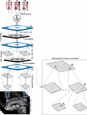
2.3 Image segmentation: HSF-CNN
The formal procedure for the proposed HSF-CNN is laid out in this section. Several existing practices need manual intervention from the operator to set their baseline parameters, reducing their precision and making them further slower. This study uses an HSF-CNN to carry out the segmentation process using dilated convolution procedures. Figure 3 depicts the overall process of the proposed HSF-CNN model.
Figure 3. HSF-CNN segmentation
The HSF-CNN works in a hierarchical manner wherein multiple layers are performed to segment the investigative RoI for AD and PD classification. When classifying cases of AD and PD, the HSF-CNN uses a multi-layer approach to segment the region of interest (RoI). The SB begins by using the usual convolution techniques to extract spatial features in a pixel-to-sub-pixel manner from the MRIs; therefore, it enables in-depth extraction of the spatial data. Each SB has three distinct extraction trails (δ1, δ2, and δ3). A (1 x 1) convolution procedure is used in three feature extraction trails to begin retrieving useful spatial characteristics. Three feature map trails, m1, m2, and m3, are generated by convolving an incoming feed with a (1 x 1) K, 'w', and 'e' as described through Eqs. (5) to (8).
$m_1=f_{\left(x_i, y_i, z_i\right)} \times w_i \pm e_i$ (5)
$m_2=f_{\left(x_i, y_j, z_j\right)} \times w_j \pm e_j$ (6)
$m_3=f_{\left(x_k, y_k, z_k\right)} \times w_k \pm e_k$ (7)
$F M=\sum\left(m_1, m_2, m_3\right)$ (8)
All the MRI scans in the records are down-sampled to retrieve spatial information effectively. In down-sampling procedures, hierarchies of SB blocks, as well as max-pooling, are used to create a smaller sample size. First, every input is fed into the initial SB block, where spatial information is extracted using a hierarchy of convolutions. Then, to lessen the operational burden on the system, the recovered features are conveyed to the max-pooling tier for image compression via dimensionality reduction. In the HSF-CNN model, the outcomes of the down-sampling tier are fed into the subsequent up-sampling tier, which is responsible for isolating the potentially suspect areas in the b-MRI scans for the segmentation of AD or PD.
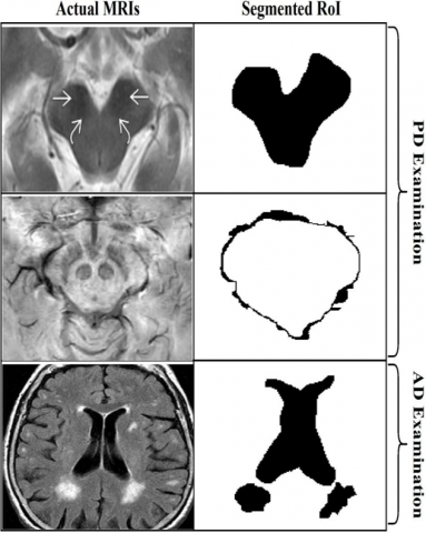
After features are captured using down-sampling, they are sent to the up-sampling tier to be handled to decode/boost the dimensions of the vital feature. This method boosts the spatial aspect by performing un-pooling techniques on the result produced from the down-sampling tier. To retrieve various spatial information using hierarchical convolutions, they are sent into the final SB block for processing. Ultimately, the up-sampling tiers' final features are extracted with the help of the SB-blocks' output, which is then passed into an un-pooling tier to boost the dimensions of the crucial features. To acquire MRI interpretations, both sampling tiers provide several granularity options. To estimate the likelihood of the target class in the input image, a sigmoid function is added to the result of the final up-sampling tier. Figure 4 highlights the effectiveness and significance of the proposed model via some sample segmented images.
Figure 4. Sample segmented images using HSF-CNN
2.4 Grad-CAM classification
Much research has postulated that CNN's more profound interpretations can capture the finest high-level structures. In addition, CNN automatically retrains a few essential spatial data points that were dropped off in the fully-connected networks so that researchers may prioritize the ideal tradeoff among distinct spatial features and high-level interpretations in the final convolution operation.
Thus, to overcome such issues we incorporated Grad-CAM in the proposed model to classify the disorders. In contrast to CAM, Grad-CAM analyses each convolutional neuron towards a decision using the gradient data passing into the CNN's final layer (convoluted). To acquire the category-oriented discriminatory localized mapping with dimensions of ѱ and h for objective class c, it is essential to compute the gradient score for any c, relevant feature mapping of a convolutional layer. The 'W' assigned to neurons in the class label is derived from a global average pooling of the gradients riposting from those neurons.
The 'ƥw' assigned to each neuron is determined by taking a multilateral aggregate of the gradients that are streaming back along the ѱ and h dimensions. All the computation processes are referred from [40] and integrated the computation into the proposed model.
$ƥ_k^c=\left(\frac{1}{P}\right) \sum i \sum j\left[\partial s^c / \partial \mathbb{A}_{i j}^k\right]$ (9)
where, $ƥ_k^c$ also referred to as partial linearization, ' P ' denotes the pixel of the processing MRI, $\mathbb{A}^{\mathrm{k}}$ represents the feature map activation in ${\partial} {s}^{{c}} / {\partial} \mathbb{A}_{i j}^{{k}}$, k denotes the feature maps, and $\mathrm{S}^{\mathrm{C}}$ refers to the score of c (before softmax).
During the process of computing $ƥ_k^c$ for c, when back-propagating gradients are conditioned to $\mathbb{A}^k$, the exact calculation corresponds to consecutive vector combinations of the connection weights as well as the gradient to the actual convolution operation from which the variations are being propagated. This continues until the gradients reach their ultimate destination using the ultimate convolution operation.
Following the determination of $ƥ_k^c$ for the c, a final class discriminative map is generated by a weighted mixture of $\mathbb{A}^k$and ReLU, as shown by the expression in Eq. (10):
$\mathbb{F}_{ {gradCAM }}^c={ReLU}\left[\sum\left(ƥ_k^c\right) \cdot\left(\mathbb{A}^k\right)\right]$ (10)
Figure 5. Workflow of Grad-CAM
Grad-CAM generates a heat-map representation of the "c" for a specified classification. Such a heat map may be used by researchers or practitioners to compositionally confirm the region of the disorders on which CNN is focusing. The grad-CAM method is reflected as algorithms in Table 2. Figure 5 provides a visual representation of the workflow required to perform all deep-learning tasks.
Table 2. Algorithm of Grad-CAM process
|
Step 1: Compute $s^c$ conditioned to $\mathbb{A}^{\mathrm{k}}$ in $\left[ {\partial s ^ { c }} / {\partial} \mathbb{A}_{i j}^k\right]$ |
|
Step 2: Equate global average pooling to retrieve, $ƥ_k^c$ |
|
$ƥ_k^c=\left(\frac{1}{P}\right) \sum i \sum j\left[\partial s^c / \partial \mathbb{A}_{i j}^k\right]$ |
|
Step 3: Compute the ultimate Grad-CAM discriminative map of 'c |
|
$\mathbb{F}_{ {gradCAM }}^c={ReLU}\left[\sum\left(ƥ_k^c\right) \cdot\left(\mathbb{A}^k\right)\right]$ |
The CNN classifier's training allows it to create CAMs from either typical or aberrant ROIs through the Grad-CAM technique. These CAMs serve as masking, revealing only the relevant features for categorization purposes.
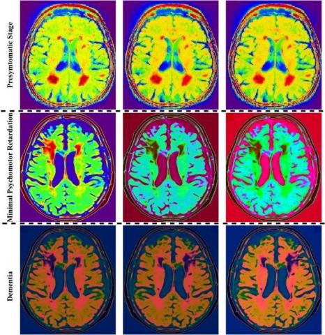
Contrasting other interpretation methods like BCFCM, SOM-based approach, and area-based ACM, the Grad-CAM-based procedures are fully model interoperable. Figure 6 and Figure 7 display the generated heat maps, which are classified according to the three stages of AD (presymptomatic, minor psychomotor impairment, and dementia) and the two major stages of PD (primary and secondary symptomatic stages), respectively. A close examination of the maps reveals that the suggested HSF-CNN significantly aided in the categorization of AD and PD. Furthermore, due to the utilization of diverse areas for sensitivity assessment, the heat maps are consistent and reliable. As a whole, the HSF-CNN segmentation approach accurately finds discriminative areas and supports Grad-CAM in classifying the disease at different phases based on the available b-MRIs. Figures 6 and 7 depict some of the significant heat-map images of both AD and PD to showcase the effectiveness of Grad-CAM.
Of particular significance are the best GRAD-CAM-trained CNN networks for producing heat maps to analyze the effect of MRI characteristics from each given layer on categorization. There is a close connection between retrieved characteristics from RoI and disorder pathogenesis, as seen by the distinctive patterns in AD and PD heat maps. Based on our findings, we conclude that there were significant differences in the heatmap trends across the categories. We validated our patient data set right away and regulated it based on their characteristics and clinical similarities. Consequently, it is realistic to predict the identification of structural variations across different cohorts.
Furthermore, it was unknown exactly where and to what extent the variances would exist within a given domain. An innovative way to investigate this problem is to use heatmap approaches inside a CNN. According to the findings of our leading HSF-CNN models and Grad-CAM, the main discriminative regions of MRI have a significantly wider range of influence than previously thought. In addition, the quantifiable Grad-CAM analysis revealed higher 90thpercentile scores, which the heat map interprets as indicating more widespread abnormalities.
Figure 6. Categorized samples of ADs in CAM filtered MRIs using Grad-CAM algorithm
Figure 7. Categorized samples of PDs in CAM filtered MRIs using Grad-CAM algorithm
(RoI: Substantia Nigra)
Specificity, sensitivity, and precision are three metrics often used to assess the efficacy of diagnostic image analysis strategies. Thus, they have been applied in our study to assess whether the suggested unique HSF-CNN segmentation approach works in tandem with the Grad-CAM classification methodology. Any methodology's sensitivity can be calculated by dividing the number of correct results by the combined number of correct and incorrect results. In other words, this is the proportion of actual positives that can be reliably detected using the recommended approach. Nonetheless, specificity is defined as the proportion of actual negative results relative to the combined true positive and actual negative results. Specificity and sensitivity are determined by employing the appropriate formulas, which are referred from study [41].
On the other hand, the precise completeness of the segmented outcomes is evaluated to assess how accurate the suggested approach is. It's a finding that considers both how sensitive and specific a test is. Thus, the specificity outcome from Figure 8 reveals that the proposed model has a high capacity to detect the disorder from the MRIs. High specificity values, close to one, indicate a strong ability to distinguish the background from the RoI, as a large number of voxels are correctly identified as background.
Figure 8. Analysis of (a) Specificity (b) Sensitivity (c) Classification accuracy
HSF-CNN is used for segmentation to enhance the Grad-CAM classification technique. The HSF-CNN+Grad-CAM-based classifier uses the concept of reducing the limitations on the inaccuracy created by the classification algorithm over the testing dataset that wasn't utilized throughout learning, allowing it to successfully classify visuals that were not part of the training phase. In the suggested technique, we use HSF segmentation to extract detailed spatial characteristics for classifying data. CNN-based classification and Grad-CAM analysis are the two main components of the classification phase. The input consists of the visual aspects and their associated labeled output. The generated outcome from Figure 8 exhibits a strategy that uses such characteristics to estimate the associated label. After using HSF-CNN, we found that our classifier's performance correctness increased from 92.13% to 98.17%. Consequently, the findings of this research signify the relevance and importance of the suggested model to the Grad-CAM-assisted classification model. Figure 9 demonstrates the effectiveness of the proposed model via the segmentation effect.
Figure 9. Analysis of segmentation effect on classification accuracy
Furthermore, the acquired MRIs are examined with their test dataset visuals to evaluate the effectiveness of the suggested approach for PD and AD classification. To measure how well a model works, statisticians use the MCC, which is derived from the contingency table. MCC is employed to assess the accuracy of binary categorization. From the contingency table, the MCC may be determined by the formula provided by the study [42]. It gives a number ranging from -1 (an erroneous classification) to +1 (a proper classification). Table 3 shows that the suggested model performs well for many different b- MRI types (T1, T2, and Flair).
Table 3. MCC metric results of different approaches
|
MRI |
HSF-CNN+Grad-CAM |
SOM-Based |
Area-Based |
BAFCM |
|
T1 |
0.92±0.13 |
0.89± 0.21 |
0.82±0.32 |
0.86±0.21 |
|
T2 |
0.98±0.25 |
0.87± 0.57 |
0.79±0.41 |
0.87±0.34 |
|
Flair |
0.95±0.37 |
0.91± 0.44 |
0.83±0.23 |
0.84±0.11 |
Figure 10 shows ROC curves for four distinct approaches used to classify ROIs in b- MRI scans. AUC values of 0.872 for BCFCM, 0.811 for the SOM-based approach, 0.792 for the area-based approach, and 0.943 for the suggested HSF-CNN+Grad-CAM show that the present approaches yield comparatively poor classification results. The suggested model performs categorization utilizing the appropriate outputting principle features, which improves classification accuracy by incorporating all of the aforementioned MRI characteristics.
Figure 10. ROC curves for AD and PD classification using various MRIs (a) T1 (b) T2 (c) FLAIR
This study is limited in some aspects including
In this research, we create a novel method using HSF-CNN for segmentation and Grad-CAM for classifying PD and AD from existing b-MRIs. To verify the effectiveness of the new model, it is compared to a limited number of existing methods. Each method provides insights into the improvement of the categorization process. Yet they are limited in a multitude of aspects. The core concern of this research is to develop and analyze a feasible b-MRI segmentation strategy and classification method for the early diagnosis of PD and AD with high accuracy. HSF-CNN is a segmentation method that enhances the Grad-CAM classification technique. The HSF-CNN divides the researchable RoI for Alzheimer's and Parkinson's disease hierarchically. In Grad-CAM, the last convolutional layer of a CNN is fed gradient information, which is then used to assign prioritization weights to each neuron depending on its impact on the preference of concern. Therefore, the classification issues arising from PD and AD are addressed using the Grad-CAM with CNN. Extensive studies showed that the proposed model outperforms other current models in terms of classification accuracy, with our best results reaching over 98.17%. The study's findings can be applied to segmenting a wide variety of medical imagery visuals for diagnosing any disorders. Further this study should be analyzed using multi-modal datasets for extracting more informative features to enhance the performance of classification of these diseases. We intend to build an automated smart communication system to support all of the domain's stakeholders in the future.
|
2D |
Two-Dimensional |
|
3D |
Three-Dimensional |
|
ACM |
Active Contour Model |
|
AD |
Alzheimer Diseases |
|
AHE |
Adaptive Histogram Equalization |
|
AUC |
Area Under Curve |
|
BCFCM |
Bias Corrected Fuzzy C-Means |
|
b-MRI |
Brain-MRI |
|
CAM |
Class Activation Mapping |
|
CNN |
Convolutional Neural Network |
|
CT |
Computerized Tomography |
|
EM |
Expectation-Maximization |
|
ET |
Emission Tomography |
|
FCM |
Fuzzy C-Means |
|
FLAIR |
Fluid Attenuated Inversion Recovery |
|
FM |
Feature Map of the ithpixel |
|
Grad-CAM |
Gradient-weighted Class Activation Mapping |
|
GDF |
Gaussian Density Function |
|
HE |
Histogram Equalization |
|
HSF |
Hierarchical Spatial Features |
|
INU |
Intensity Non-Uniformity |
|
K |
Kernel |
|
K-L |
Kullback-Leibler |
|
MAP |
Maximum-a-Posterior |
|
MCC |
Mathews Correlation Coefficient |
|
MR |
Magnetic Resonance |
|
MRF |
Markov Random Field |
|
MRI |
Magnetic Resonance Imaging |
|
NN |
Neural Network |
|
OCT |
Optical Coherence Tomography |
|
PD |
Parkinson Diseases |
|
|
Probability Density Function |
|
RF |
Radio Frequency |
|
RFC |
Relative Fuzzy Connectedness |
|
ROC |
Receiver Operator Characteristic |
|
RoI |
Region of Interest |
|
SB |
Spatial Block |
|
SNR |
Signal-to-Noise Ratio |
|
SOM |
Self-Organizing Map |
[1] Mahesh, T.R., Vinoth Kumar, V., Vivek, V., Karthick Raghunath, K.M., Sindhu Madhuri, G. (2022). Early predictive model for breast cancer classification using blended ensemble learning. International Journal of System Assurance Engineering and Management. https://doi.org/10.1007/s13198-022-01696-0
[2] Jiang, T., Sun, Q., Chen, S. (2016). Oxidative stress: A major pathogenesis and potential therapeutic target of antioxidative agents in Parkinson’s disease and Alzheimer’s disease.Progress in Neurobiology, 147: 1-19. https://doi.org/10.1016/j.pneurobio.2016.07.005
[3] Kalia, L.V., Lang, A.E. (2015). Parkinson’s disease. The Lancet, 386(9996): 896-912. https://doi.org/10.1016/s0140-6736(14)61393-3
[4] Hesamian, M.H., Jia, W., He, X., Kennedy, P. (2019). Deep Learning Techniques for Medical Image Segmentation: Achievements and Challenges. Journal of Digital Imaging, 32(4): 582-596. https://doi.org/10.1007/s10278-019-00227
[5] Umamaheswaran S., John, R., Nagarajan S., Karthick Raghunath K.M., Arvind K.S. (2022). Predictive Assessment of Fetus Features Using Scanned Image Segmentation Techniques and Deep Learning Strategy. International Journal of E- Collaboration, 18(3): 1-13. https://doi.org/10.4018/ijec.307130
[6] Xia, M., Yan, W., Huang, Y., Guo, Y., Zhou, G., Wang, Y. (2019). IVUS Image Segmentation Using Superpixel-Wise Fuzzy Clustering and Level Set Evolution. Applied Sciences, 9(22): 4967. https://doi.org/10.3390/app9224967
[7] Jayaraman, S, Esakkirajan, S., Veerakumar, T. (2013), Digital Image Processing. McGraw Hill Education Pvt Limited.
[8] Priyadarshi, N., Bhoi, A.K., Padmanaban, S., Balamurugan, S., Holm-Nielsen, J.B. (2022). Intelligent renewable energy systems: integrating artificial intelligence techniques and optimization algorithms. Wiley-Scrivener. https://doi.org/10.1002/9781119786306
[9] Umbaugh, S.E., Wei, Y.S. Zuke, M. (1997). Feature extraction in image analysis. A program for facilitating data reduction in medical image classification. IEEE Engineering in Medicine and Biology Magazine, 16(4): 62-73. https://doi.org/10.1109/51.603650
[10] Suganya, A., Aarthy, S.L. (2022). Alzheimer's And Parkinson's Disease Classification Using Deep Learning Based On MRI: A Review. International Journal of Communication Networks and Information Security, 14(1s): 9-21. https://doi.org/10.17762/ijcnis.v14i1s.5588
[11] Kaplan, E., Altunisik, E., Firat, Y.E., Barua, P.D., Dogan, S., Baygin, M., Acharya, U.R. (2022). Novel nested patch-based feature extraction model for automated Parkinson's Disease symptom classification using MRI images. Computer Methods and Programs in Biomedicine, 224: 107030. https://doi.org/10.1016/j.cmpb.2022.107030
[12] Broich, K. (2009). Committee for Medicinal Products for Human Use (CHMP) assessment on efficacy of antidepressants. European Neuropsychopharmacology, 19(5): 305-308. https://doi.org/10.1016/j.euroneuro.2009.01.012
[13] Tishchenko, I., Riveros, C., Moscato, P. (2016). Alzheimer’s disease patient groups derived from a multivariate analysis of cognitive test outcomes in the Coalition Against Major Diseases dataset. Future Science OA, 2(3): FSO140. https://doi.org/10.4155/fsoa-2016-0041
[14] Rohrer, J.D., Nicholas, J.M., Cash, D.M., van Swieten, J., Dopper, E., Jiskoot, L., van Minkelen, R., Rombouts, S.A., Cardoso, M.J., Clegg, S., Espak, M., Mead, S., Thomas, D.L., De Vita, E., Masellis, M., Black, S.E., Freedman, M., Keren, R., MacIntosh, B.J., Rogaeva, E. (2015). Presymptomatic cognitive and neuroanatomical changes in genetic frontotemporal dementia in the Genetic Frontotemporal dementia Initiative (GENFI) study: a cross-sectional analysis. The Lancet Neurology, 14(3): 253-262. https://doi.org/10.1016/s1474-4422(14)70324-2
[15] Vovk, U., Pernuš, F., Likar, B. (2006). Intensity inhomogeneity correction of multispectral MR images. NeuroImage, 32(1): 54-61. https://doi.org/10.1016/j.neuroimage.2006.03.020
[16] Belaroussi, B., Milles, J., Carme, S., Zhu, Y.M., Benoit-Cattin, H. (2006). Intensity non- uniformity correction in MRI: Existing methods and their validation. Medical Image Analysis, 10(2): 234-246. https://doi.org/10.1016/j.media.2005.09.004
[17] Lötjönen, J. MP., Wolz, R., Koikkalainen, J. R., Thurfjell, L., Waldemar, G., Soininen, H., Rueckert, D. (2010). Fast and robust multi-atlas segmentation of brain magnetic Resonance images. NeuroImage, 49(3): 2352-2365. https://doi.org/10.1016/j.neuroimage.2009.10.026
[18] Artaechevarria, X., Munoz-Barrutia, A., Ortiz-de-Solorzano, C. (2009). Combination Strategies in Multi-Atlas Image Segmentation: Application to Brain MR Data. IEEE Transactions on Medical Imaging, 28(8): 1266-1277. https://doi.org/10.1109/tmi.2009.2014372
[19] Jia, H., Yap, P.T., Shen, D. (2012). Iterative multi-atlas-based multi-image segmentation with tree-based registration. NeuroImage, 59(1): 422-430. https://doi.org/10.1016/j.neuroimage.2011.07.036
[20] Wang, H., Yushkevich, P.A. (2013). Multi-atlas segmentation with joint label fusion and corrective learning—an open source implementation. Frontiers in Neuroinformatics, 7. https://doi.org/10.3389/fninf.2013.00027
[21] Yan, B., Xie, M., Gao, J.J., Zhao, W. (2010). A fuzzy C-means-based algorithm for bias field estimation and segmentation of MR images. The 2010 International Conference on Apperceiving Computing and Intelligence Analysis Proceeding. https://doi.org/10.1109/icacia.2010.5709907
[22] Yang, X., Fei, B. (2011). A multiscale and multiblock fuzzy C-means classification method for brain MR images. Medical Physics, 38(6Part1): 2879-2891. https://doi.org/10.1118/1.3584199
[23] Ji, Z., Sun, Q., Xia, Y., Chen, Q., Xia, D., Feng, D. (2012). Generalized rough fuzzy c- means algorithm for brain MR image segmentation. Computer Methods and Programs in Biomedicine, 108(2): 644-655. https://doi.org/10.1016/j.cmpb.2011.10.010
[24] Ahmed, M.N., Yamany, S.M., Mohamed, N., Farag, A.A., Moriarty, T. (2002). A modified fuzzy c-means algorithm for bias field estimation and segmentation of MRI data. IEEE Transactions on Medical Imaging, 21(3): 193-199. https://doi.org/10.1109/42.996338
[25] Demirhan, A., Güler, İ. (2011). Combining stationary wavelet transform and self-organizing maps for brain MR image segmentation. Engineering Applications of Artificial Intelligence, 24(2): 358-367. https://doi.org/10.1016/j.engappai.2010.09.008
[26] Ortiz, A., Górriz, J.M., Ramirez, J., Salas-Gonzalez, D. (2011). MR brain image segmentation by growing hierarchical SOM and probability clustering. Electronics Letters, 47(10): 585-586. https://doi.org/10.1049/el.2011.0322
[27] McIntosh, C., Hamarneh, G. (2017). Medical image segmentation: Energy minimization and deformable models. Medical Imaging, 661-692. https://doi.org/10.1201/b15511- 23
[28] Wang, L., Li, C., Sun, Q., Xia, D., Kao, C.Y. (2009). Active contours driven by local and global intensity fitting energy with application to brain MR image segmentation. Computerized Medical Imaging and Graphics, 33(7): 520-531. https://doi.org/10.1016/j.compmedimag.2009.04.010
[29] Moreno, J.C., Surya Prasath, V.B., Proença, H., Palaniappan, K. (2014). Fast and globally convex multiphase active contours for brain MRI segmentation. Computer Vision and Image Understanding, 125: 237-250. https://doi.org/10.1016/j.cviu.2014.04.010
[30] Zheng, Q., Dong, E., Cao, Z., Sun, W., Li, Z. (2014). Active contour model driven by linear speed function for local segmentation with robust initialization and applications in MR brain images. Signal Processing, 97: 117-133. https://doi.org/10.1016/j.sigpro.2013.10.008
[31] Rudra, A.K., Sen, M., Chowdhury, A.S., Elnakib, A., El-Baz, A. (2011). 3D Graph cut with new edge weights for cerebral white matter segmentation. Pattern Recognition Letters, 32(7): 941-947. https://doi.org/10.1016/j.patrec.2010.12.013
[32] Ciesielski, K.C., Miranda, P.A.V., Falcão, A.X., Udupa, J.K. (2013). Joint graph cut and relative fuzzy connectedness image segmentation algorithm. Medical Image Analysis, 17(8), 1046-1057. https://doi.org/10.1016/j.media.2013.06.006
[33] Scherrer, B., Forbes, F., Garbay, C., Dojat, M. (2009). Distributed Local MRF Models for Tissue and Structure Brain Segmentation. IEEE Transactions on Medical Imaging, 28(8): 1278-1295. https://doi.org/10.1109/tmi.2009.2014459
[34] Lowry, N., Mangoubi, R., Desai, M., Marzouk, Y., Sammak, P. (2011). A unified approach to expectation-maximization and level set segmentation applied to stem cell and brain MRI images. 2011 IEEE International Symposium on Biomedical Imaging: From Nano to Macro. https://doi.org/10.1109/isbi.2011.5872672
[35] Kumar, S., Ray, S.K., Tewari, P. (2012). A hybrid approach for image segmentation using fuzzy clustering and level set method. International Journal of Image, Graphics and Signal Processing, 4(6): 1-7. https://doi.org/10.5815/ijigsp.2012.06.01
[36] Wang, L., Shi, F., Yap, P.T., Lin, W., Gilmore, J.H., Shen, D. (2013). Longitudinally guided level sets for consistent tissue segmentation of neonates. Human Brain Mapping, 34(7): 1747-1747. https://doi.org/10.1002/hbm.22325
[37] Suganya, A., Aarthy, S.L. (2023). Application of deep learning in the diagnosis of alzheimer's and parkinson's disease-a review. Current Medical Imaging. https://doi.org/10.2174/1573405620666230328113721
[38] Jadwa, S.K. (2018). Wiener filter based medical image de-noising. International Journal of Science and Engineering Applications, 7(9): 318-323. https://doi.org/10.7753/ijsea0709.1014
[39] Padmavathy, V., Priya, D. (2018). Image contrast enhancement techniques-a survey. International Journal of Engineering & Technology, 7(3.3): 466. https://doi.org/10.14419/ijet.v7i2.33.14811
[40] Selvaraju, R.R., Cogswell, M., Das, A., Vedantam, R., Parikh, D., Batra, D. (2020). Grad- CAM: Visual explanations from deep networks via gradient-based localization. International Journal of Computer Vision, 128(2): 336-359. https://doi.org/10.1007/s11263-019-01228-7
[41] Müller, D., Soto-Rey, I., Kramer, F. (2022). Towards a guideline for evaluation metrics in medical image segmentation. BMC Research Notes, 15(1). https://doi.org/10.1186/s13104-022-06096-y
[42] Subbanna, N., Wilms, M., Tuladhar, A., Forkert, N.D. (2021). An analysis of the vulnerability of two common deep learning-based medical image segmentation techniques to model inversion attacks. Sensors, 21(11): 3874. https://doi.org/10.3390/s21113874