Xinying Zhang![]() | Lang Li
| Lang Li![]() | Chuannan Fu
| Chuannan Fu![]() | Xixi Han*
| Xixi Han*![]()
© 2023 IIETA. This article is published by IIETA and is licensed under the CC BY 4.0 license (http://creativecommons.org/licenses/by/4.0/).
OPEN ACCESS
Classical frequency measurement techniques, such as direct frequency measurement, multi-cycle synchronous frequency measurement, analog interpolation, time-amplitude conversion, and the cursor method, predominantly rely on hardware, necessitating high hardware standards and potentially leading to measurement errors. These hardware-induced errors pose significant challenges in enhancing measurement precision. To address this issue, a novel frequency measurement methodology employing Lissajous figures is investigated in this study. The frequency of a given signal is obtained by measuring the flipping period of Lissajous figures using a reading frequency approach. As the implementation of Lissajous figures is carried out within the LabVIEW environment, traditional hardware constraints are circumvented, eliminating associated errors and resulting in increased precision in frequency measurement. Moreover, an image matching technique is utilized to accurately determine the flipping period, further improving the precision of the obtained frequency value. The introduction of this innovative method offers a fresh perspective in the field of frequency measurement, enhancing the potential for more accurate measurements. Although continued research is warranted to explore the expansion and refinement of this technique, it holds promise for promoting advancements within the field. This approach demonstrates potential benefits not only for frequency measurement but also for a wide range of scientific and engineering applications.
Lissajous figures, frequency measurement, flipping period, image matching
As time and frequency technology advances, including enhancements in the accuracy of time and frequency standard sources, and an ever-expanding scope of applications, the demands for time and frequency measurement have grown [1, 2]. Instruments designed using various existing methods each possess their own merits and drawbacks. Some offer high accuracy but have a narrow frequency measurement range, while others meet measurement requirements but exhibit complex structures and high costs. Consequently, proposing a simple and practical measurement method by combining existing techniques and the periodic characteristics of time and frequency signals is of significant research value.
The direct frequency measurement method, also known as the pulse filling method, has been utilized by Jiang et al. [3]. Its principle involves filling pulses into a given gate signal, obtaining the number of filled pulses through counting circuits, and calculating the frequency of the signal to be measured. This method boasts advantages such as simple equipment, small size, low cost, and easy measurement. However, drawbacks include an error of ±1 count during frequency measurement in the counting circuit. To achieve higher measurement accuracy, a high measurement frequency and a sufficiently long gate signal time are required, resulting in lower accuracy for low measured frequencies. The multi-cycle synchronous frequency measurement method [4, 5] eliminates the ±1 count error but cannot continuously measure and requires a high standard frequency for fast measurement. This leads to a relatively large number of bits when counting the standard frequency and consumes considerable hardware resources. The analog interpolation method [6-8], which measures time intervals for frequency measurement, improves the resolution by three orders of magnitude but does not eliminate the ±1 count error. Furthermore, it suffers from long conversion times and difficulties in controlling nonlinearity. The time-amplitude conversion method [9] overcomes the problems of the analog interpolation method by replacing the discharge current source in the measurement circuit with a high-speed A/D converter and a reset circuit. The cursor method [10, 11], based on a principle similar to mechanical vernier calipers, measures the fractional part and tail number of the whole cycle more accurately, improving measurement accuracy and resolution. Nonetheless, the cursor method entails a relatively complex measurement circuit technology and long conversion times.
The Lissajous figure frequency measurement method [12-14] connects the measured frequency signal and the known frequency standard signal to the x-axis and y-axis of the cathode ray oscilloscope, respectively. The standard signal frequency is adjusted, and the measured signal frequency is determined according to the Lissajous figure and the known signal frequency. Most existing measurement methods are implemented through hardware, necessitating high hardware requirements to achieve relatively high measurement accuracy. It is challenging to eliminate errors caused by hardware in practical applications, leading to issues with improving measurement accuracy due to hardware errors. The present study proposes a novel calculation method for the flipping period of Lissajous figures. This new method determines the measured frequency through the flipping period based on the principle of image processing, using the normalized gray-scale matching method to process the video of Lissajous figures, obtaining the flipping period of the figures, and subsequently calculating the value of the measured frequency. Since Lissajous figures are implemented in LabVIEW, they are not constrained by hardware in traditional frequency measurement methods, eliminating errors caused by hardware in traditional measurement methods and improving frequency measurement accuracy.
Research on frequency measurement methods based on Lissajous figures holds great significance for the field of frequency measurement. In today's rapidly advancing information technology landscape, investigating high-accuracy frequency measurement is an essential aspect related to economic development, technological innovation, and national security [15].
Figure 1. Measurement scheme for flipping period of Lissajous figures
2.1 Measurement scheme for frequency measurement method based on Lissajous figures
Image matching refers to the recognition of homonymous points between images through a certain matching algorithm. According to the different methods of selecting matching features, matching methods can be divided into two categories: gray-scale-based and feature-based [16-18]. In this study, the normalized gray-scale matching method is used. The measurement scheme for obtaining the flipping period of Lissajous figures using image matching algorithms is shown in Figure 1. After obtaining the Lissajous figures in LabVIEW, a camera is used to capture the video of Lissajous figures, which is then input into MATLAB. The image matching algorithm is used to estimate the flipping period of Lissajous figures, and the frequency difference between the standard signal and the measured signal is derived using formulas to obtain the frequency of the measured signal.
2.2 Simulation system design based on LabVIEW
The software processing process of the frequency measurement method based on Lissajous figures is mainly implemented by LabVIEW. This process consists of two parts: the first part is to control the Agilent U2702A modular oscilloscope using LabVIEW, and the second part is to display the Lissajous figures of the two input signals on the computer.
LabVIEW uses the graphical programming language G to create programs, which are generated in a block diagram format, while other computer languages generate code based on text-based languages [19]. LabVIEW software is the core of the NI design platform and is the ideal choice for developing measurement or control systems.
Figure 2. System Block Diagram of the simulation system based on LabVIEW
Figure 3. Simulation system based on LabVIEW
The signal source of the simulation system based on LabVIEW is the standard signal from the crystal oscillator and the sine signal generated by the frequency signal generator Agilent 8644A. They are processed by NI LabVIEW2014 programming on a computer, and the Lissajous figures of the two signals are displayed on the LabVIEW front panel. According to the formula, the value of the measured signal is obtained from the flipping period of Lissajous figures.
The system block diagram of the simulation system based on LabVIEW is shown in Figure 2. The standard frequency sent by the reference module and the measured frequency sent by the measured module are input to two ports of the modular oscilloscope. The signals are converted into signals that LabVIEW can receive and combined into Lissajous figures in LabVIEW. After software processing, the measured frequency is obtained.
The experimental scene of the simulation system based on LabVIEW is shown in Figure 3, which is mainly implemented by the Agilent U2702A modular oscilloscope, frequency signal generator Agilent 8644A, and a computer equipped with NI LabVIEW.
3.1 LabVIEW programming process
3.1.1 LabVIEW controlling Agilent U2702A modular oscilloscope
(1) Create a connection with the IVI-COM driver
Follow these steps in NI LabVIEW to use the IVI-COM driver:
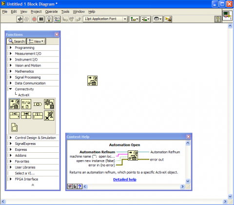
a. Start LabVIEW and open a blank VI. Two windows appear, the front panel window and the block diagram window.
b. Locate the Automation Open icon in the Connectivity >> ActiveX function panel and drag it to the block diagram window, as shown in Figure 4.
Figure 4. Placing Automation Open in the block diagram
Figure 5. Adding IVI driver library
c. Right-click on the first terminal (Automation Refnum) on the left side of the Automation Open icon and select Select ActiveX Class >> Browse.
d. From the Type Library panel's dropdown menu, choose IVI KeysightU2701A Type Library Version 1.0, as shown in Figure 5.
e. From the object hierarchy tree, select IAgilentU2701A, as shown in Figure 6.
f. Click OK to return to the block diagram window. The Automation Refnum terminal connects to AgilentU2701ALib.IAgilentU2701A, as shown in Figure 7.
g. Right-click on the last terminal (error in - (no error)) on the left side of the Automation Open icon and select Create >> Control, as shown in Figure 8.
Figure 6. Selecting IAgilentU2701A
Figure 7. Connecting terminals
Figure 8. Connecting terminals
(2) Using the driver
Call Initialize to establish a connection with Keysight U2701A / U2702A, and call Close to terminate the connection. Follow these steps to initialize the instrument, use it, and close the connection after use:
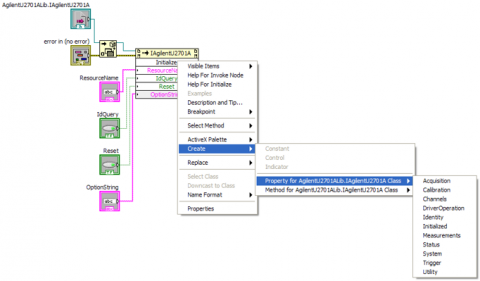
a. Locate the Invoke Node icon in the Functions panel Connectivity >> ActiveX and drag it to the block diagram, as shown in Figure 9.
b. Right-click on the Property Node icon and select Select Class >> ActiveX >> AgilentU2701ALib.IAgilentU2701A.
c. Connect the terminals as shown in Figure 10.
d. Click on the Method icon and select Initialize, as shown in Figure 11.
e. Create appropriate controls for all input terminals on the left side by right-clicking each terminal and selecting Create >> Control. Obtain the instrument's Resource Name using the Keysight Connection Expert. Find the Keysight U2701A / U2702A and resource name under the VISA address in the USB interface, as shown in Figure 12 (red circle) (USB0::2391::10520::MY48151002::0::INSTR).
f. The VISA address can also be obtained from the National Instrument Measurement and Automation Explorer, as shown in Figure 13 (red circle).
Figure 9. Placing Invoke Node in the block diagram
Figure 10. Connecting terminals
Figure 11. Clicking on the Method icon and selecting Initialize
Figure 12. Finding the instrument's VISA address method 1
Figure 13. Finding the instrument's VISA address method 2
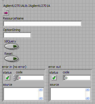
g. After creating all the controls, the front panel and block diagram appear as shown in Figures 14 and 15.
Front panel:
Figure 14. Front panel
Block diagram:
Figure 15. Block diagram
h. Continue program development by right-clicking on the Initialize icon and selecting Create, as shown in Figure 16.
Figure 16. Continuing program development
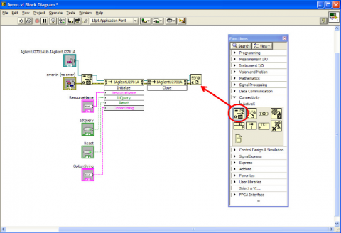
i. Complete the program by right-clicking on the last icon and selecting Create. Select the Close method and connect the corresponding terminals. The block diagram appears as shown in Figure 17.
Figure 17. Block diagram
j. Locate the Close Reference icon in the Connectivity >> ActiveX panel and drag it to the block diagram. Connect the terminals as shown in Figure 18.
Figure 18. Terminal connections
k. Create an error output indicator by right-clicking the Close Reference icon terminal and selecting Create >> Indicator. The front panel and block diagram appear as shown in Figures 19 and 20.
l. For convenience or personal preference, right-click on each control and indicator and deselect View As icon, as shown in Figure 21.
m. The block diagram will appear as shown in Figure 22.
Figure 19. Front panel
Figure 20. Block diagram
Figure 21. Simplifying icons
Figure 22. Simplified block diagram after removing icons
The complete example demonstrates the steps required to identify the instrument, reset the instrument, automatically measure the instrument, perform a simple measurement, and finally acquire and save waveform data. The complete example front panel is shown in Figure 23.
Figure 23. Complete example front panel
3.1.2 Displaying Lissajous figures in LabVIEW
Figure 24. Adding another signal to the block diagram
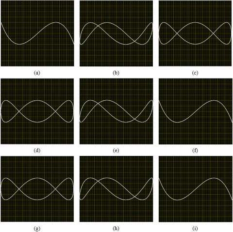
Figure 25. Lissajous figures at different moments with frequency deviation
To obtain Lissajous figures, the test frequency signal and standard frequency signal must be fed into the oscilloscope's Y-axis input and X-axis input, respectively. It is necessary to provide two input signals simultaneously to the modular oscilloscope U2702A. After obtaining a complete program that acquires and displays one waveform, another signal should be added to the block diagram after the AutoSetup to acquire two waveforms. The specific block diagram is shown in Figure 24.
The subsequent program is consistent with the program for inputting one signal. After adding another signal and completing the input of both signals, place the Express XY control on the front panel to complete the input and display of the two signals. Connect the X input and Y input on the left side of the created XY graph, paying attention to data types to prevent connection errors that cause the program to fail.
Figure 25 shows the Lissajous figure when the frequency ratio is and there is a slight frequency deviation. As can be seen from the figure, starting from the initial moment (a), the Lissajous figure goes through the process of (b) - (h) and eventually returns to the initial moment (i). (a) and (i) are the same. In this case, the time experienced from (a) to (i) is called a rotation period. After obtaining the value of the rotation period, the frequency difference can be determined.
4.1 Image processing method
A video is composed of many consecutive frames, each of which is actually an image. The time interval between two adjacent frames is inversely proportional to the frame rate. Randomly set a frame in the video as the starting frame of the rotation period. If the ending frame can be found, then calculate the time interval between the starting frame and ending frame to obtain the period value of the Lissajous figure. The key to the algorithm is how to determine the starting frame and ending frame. The detailed steps of the algorithm are as follows.
First, obtain some key parameters of the video, such as resolution, frame rate, and the number of frames. Next, for the ith frame Fi(m, n) in the video, ignore the color and saturation information and keep only the brightness information, converting it into a gray-scale image I(m, n) with 256 gray levels. Segment I(m, n) to obtain the binary image J(m, n):
$J(m, n)= \begin{cases}1, & \text { if } I(m, n) \geq \text { Threshold } \\ 0, & \text { others. }\end{cases}$ (1)
Here, Threshold is the threshold value. In the binary image, pixels on the Lissajous figure and the background are represented by 1 and 0, respectively. The normalized area is defined as:
$N A_i=\frac{1}{M \times N} \sum_{m=1}^M \sum_{n=1}^N J(m, n)$ (2)
M×N represents the resolution of the video. Perform the same processing for all frames in the video to obtain the normalized area curve NA(i). Here, NOF represents the number of frames in the video.
From the normalized area curve, many negative peaks can be found. Mark the frames corresponding to these peaks. Obviously, the time interval between a marked frame and the next marked frame is the rotation period of the Lissajous figure. Suppose there are N marked frames in a video segment, and the lth marked frame is the kth frame in the video. Then, a total of N-2 period values are obtained, and the pth rotation period value is:
$\tau_p=\frac{k_{p+2}-k_p}{F R}, p=1,2, \cdots, N-2$ (3)
where, FR is the frame rate of the video.
Based on the least squares algorithm, the estimated value of the Lissajous figure's rotation period is obtained. Let the estimated value of the rotation period be ![]() , then:
, then:
$v_p=\hat{\tau}-\tau_p, p=1,2, \cdots, N-2$ (4)
Rewrite it in matrix form:
$\underset{(N-2) \times 1}{\boldsymbol{V}}=\left[\begin{array}{c}1 \\ 1 \\ \vdots \\ 1\end{array}\right] \hat{\tau}-\left[\begin{array}{c}\tau_1 \\ \tau_2 \\ \vdots \\ \tau_{N-2}\end{array}\right]=\underset{(N-2) \times 1}{\boldsymbol{B}} \hat{\tau}-\underset{(N-2) \times 1}{\boldsymbol{T}}$ (5)
Since $\tau_p$ is uncorrelated and has the same precision, according to the least squares criterion, it is required to:
$\boldsymbol{V}^T \boldsymbol{V}=\min$ (6)
Take the first derivative of the above equation with respect to ![]() and set it to 0, resulting in:
and set it to 0, resulting in:
$\frac{d \boldsymbol{V}^T \boldsymbol{V}}{d \hat{\tau}}=2 \boldsymbol{V}^T B=2 \boldsymbol{V}^T\left[\begin{array}{c}1 \\ 1 \\ \vdots \\ 1\end{array}\right]=2 \sum_{p=1}^{N-2} v_p=0$ (7)
Substitute formula (4) into the above equation:
$\sum_{p=1}^{N-2} v_p=\sum_{p=1}^{N-2}\left(\hat{\tau}-\tau_p\right)=(N-2) \hat{\tau}-\sum_{p=1}^{N-2} \tau_p=0$ (8)
Therefore:
$\hat{\tau}=\frac{1}{N-2} \sum_{p=1}^{N-2} \tau_p$ (9)
4.2 Experimental results
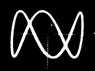
The test signal is simulated by a sine wave generated by a frequency synthesizer. Two signals are input into the Y-axis input and X-axis input of the oscilloscope, generating Lissajous figures on the oscilloscope screen. Place the camera on a tripod with the lens facing the oscilloscope screen to record the video of the Lissajous figures. To observe dynamic Lissajous figures on the oscilloscope screen, the frequency of the test signal is set as an integer multiple of 10MHz plus or minus a small frequency difference. In the experiment, the frequencies of the test signal are 10.00000220, 20.00000385, 30.0000057, 40.0000076, 50.00000955, and 60.0000116 MHz. A total of six video segments are obtained. The video resolution is 640×480, and the frame rate is 30 frames/second. Figure 26(a) shows a frame from the video obtained when the test frequency is 30.0000057 MHz. Figure 27 shows the histogram of Figure 26(b). The histogram has 256 bars, each representing the number of pixels with the same gray level. Obviously, the last peak in the histogram corresponds to the pixels on the Lissajous figure. Setting the threshold to 120-230 can achieve better segmentation results. Figure 28 shows the image segmentation result when the threshold is set to 200. From Figure 28, it can be seen that the Lissajous figure is extracted from the background noise. Calculate the normalized area of each frame in the video to obtain the normalized area curve.
Figure 26. One frame in the video
Figure 27. Histogram of Figure 26(b)
Figure 28. Image segmentation result
Figure 29 shows the normalized area curve when the test frequency is 30.0000057. From the curve, it can be seen that there are 21 negative peaks, indicating a total of 21 marked frames. In this way, 19 period values can be calculated, and then the estimated value of the rotation period can be obtained.
Table 1. Calculated mean values of Lissajous figure rotation periods
|
Frequency |
10M+2.20 |
20M+3.85 |
30M+5.7 |
40M+7.6 |
50M+9.55 |
60M+11.60 |
|
|
0.4540 0.4536 0.4546 0.4530 0.4538 0.4539 |
0.2595 0.2590 0.2600 0.2602 0.2597 0.2599 0.2600 0.2593 0.2595 0.2596 0.2600 0.2601 0.2597 0.2596 0.2594 |
0.1749 0.1753 0.1756 0.1754 0.1758 0.1760 0.1754 0.1750 0.1748 0.1752 0.1754 0.1756 0.1756 0.1750 0.1751 0.1756 0.1752 0.1761 0.1756 |
0.1310 0.1320 0.1313 0.1310 0.1313 0.1320 0.1310 0.1320 0.1317 0.1313 0.1313 0.1310 0.1315 0.1317 0.1320 0.1320 0.1315 0.1310 0.1313 0.1320 0.1317 0.1315 0.1310 0.1320 0.1310 0.1310 |
0.1045 0.1050 0.1048 0.1043 0.1044 0.1050 0.1046 0.1051 0.1050 0.1047 0.1049 0.1045 0.1045 0.1050 0.1052 0.1046 0.1048 0.1046 0.1043 0.1050 0.1048 0.1043 0.1051 0.1046 0.1050 0.1048 0.1049 0.1041 0.1041 0.1046 0.1050 0.1047 0.1046 0.1049 0.1045 0.1050 0.1043 0.1048 0.1043 0.1048 |
0.0860 0.0865 0.0862 0.0860 0.0859 0.0862 0.0860 0.0859 0.0865 0.0862 0.0862 0.0858 0.0860 0.0865 0.0864 0.0864 0.0862 0.0860 0.0858 0.0859 0.0862 0.0866 0.0862 0.0865 0.0859 0.0862 0.0865 0.0864 0.0865 0.0859 0.0864 0.0864 0.0866 0.0860 0.0858 0.0866 0.0864 0.0859 0.0864 0.0860 |
|
|
0.4538 |
0.2597 |
0.1754 |
0.1316 |
0.1047 |
0.0862 |
Figure 29. Normalized area curve
Table 1 gives the calculated mean values of the Lissajous figure rotation periods.
The 19 values of $\tau_p$ in the fourth column of Table 1 are obtained when the test frequency is 30.0000057 , and there are 21 negative peaks in the normalized area curve in Figure 29. The estimated value of the rotation period is obtained by calculating the mean value $\hat{\tau}$ of $\tau_p$. Similarly, the meanings of other columns and the fourth column are the same, all obtained by calculating the mean value $\hat{\tau}$ of $\tau_p$ to obtain the estimated value of the rotation period.
4.3 Algorithm verification
Assuming the frequency ratio of the two signals is $f_Y: f_X=m: n$ (m and n are integers), if the signal of the vertical system changes m cycles within a certain time interval, the signal of the horizontal system changes n cycles, and a stable figure will appear on the fluorescent screen. Since the signal of the vertical deflection system changes one cycle and has two intersections with the horizontal axis, m cycles have 2m intersections with the horizontal axis. Similarly, n cycles of the horizontal system signal have 2n intersections with the vertical axis.
The frequency ratio can be determined by the intersections of the Lissajous figure with the horizontal axis nX and the vertical axis nY, that is
$\frac{f_Y}{f_X}=\frac{n_X}{n_Y}$ (10)
If the known frequency signal intersects the X-axis and the test frequency signal intersects the Y-axis, then from Eq. (10), we get
$f_Y=\frac{n_X}{n_Y} \cdot f_X=\frac{m}{n} f_X$ (11)
When the ratio of the two signals' frequencies is not exactly equal to an integer ratio, but the frequency difference $\Delta f_X$ is very small, the Lissajous figure in this case is similar to the Lissajous figure when $f_Y=(m / n) f_X$.
However, due to the existence of $\Delta f_X$, it equals the phase difference between the two signals $f_x$ and $f_y$ changing continuously over time. The Lissajous figure will slowly rotate with time t. When $(\mathrm{m} / \mathrm{n}) \Delta f \cdot t=N$, it completes $N$ rotations $(N=1,2, \ldots)$. Therefore, $\Delta f$ can be determined by the time $t$ required to rotate $\mathrm{N}$ times.
From $f_Y=(m / n)\left(f_X+\Delta f_X\right)$, we know $n f_Y=m f_X+$ $m \Delta f_X$, and from the definition of the function, there is a corresponding relationship
$f\left(n f_Y\right)=f\left(m f_X+m \Delta f_X\right)$ (12)
From (12), $m \Delta f_X$ is the period of function (12), that is, the rotation period T of the Lissajous figure is
$T=\frac{1}{m \Delta f_X}$ (13)
The calculation formula for the frequency difference can be obtained from formula 13 and the previously obtained estimated value of the rotation period
$\Delta f_X=\frac{1}{m T}$ (14)
The calculation formula for the test frequency can be obtained from $n f_Y=m f_X+m \Delta f_X$ and formula 14
$f_Y=\frac{m}{n} f_X+\frac{1}{n T}$ (15)
Verify the estimated rotation period values in Table 1 with the known frequency difference according to formula 14, the results are shown in Table 2.
Table 2. Verification results
|
$T / s$ |
0.4538 |
0.2597 |
0.1754 |
0.1316 |
0.1047 |
0.0862 |
|
$\Delta f / \mathrm{Hz}$ |
2.20 |
3.85 |
5.7 |
7.6 |
9.55 |
11.60 |
|
$T=\frac{1}{m \Delta f}$ |
0.9984 |
0.9998 |
0.9998 |
1.0001 |
0.9999 |
0.9999 |
This study proposes a new Lissajous figure rotation period calculation method based on image processing technology, which uses the normalized grayscale matching method to process the video of Lissajous figures to obtain the rotation period. This method has two advantages. First, the calculation accuracy is inversely proportional to the frame rate of the video. Therefore, improving the frame rate of the video can improve the calculation accuracy. Second, the method is simple and has strong anti-interference ability. A simple image segmentation algorithm can separate the Lissajous figure from the background noise. In addition, although the segmented image contains residual coordinates, this does not affect the calculation results. The accuracy of the rotation period obtained by the normalized grayscale matching method used in this study for processing Lissajous figures with image processing algorithms is not high enough. In the next step, we will find a high-precision image processing algorithm so that the accuracy of the rotation period of the Lissajous figure will be higher, and the accuracy of the test frequency obtained will be higher.
[1] Čurović, L., Murovec, J., Novaković, T., Prezelj, J. (2022). Time–frequency methods for characterization of room impulse responses and decay time measurement. Measurement, 196: 111223. https://doi.org/10.1016/j.measurement.2022.111223
[2] Lombardi, M.A. (2006). Legal and technical measurement requirements for time and frequency. Ncsli Measure, 1(3): 60-69. https://doi.org/10.1080/19315775.2006.11721335
[3] Jiang, S., Xu, Z.Z., Tian, J., Fu, L., Zhang, K. (2021). Research on frequency testing methods for interference electrotherapy instruments. Chinese Medical Equipment Journal, 42(3): 43-50. https://doi.org/10.19745/j.1003-8868.2021051
[4] Tan, C., Wang, J., Li, Z. (2019). A frequency measurement method based on optimal multi-average for increasing proton magnetometer measurement precision. Measurement, 135: 418-423. https://doi.org/10.1016/j.measurement.2018.10.016
[5] Hao, Y.Z., Zhou, Q. (2016). Lag error analysis and improvement of the dynamic frequency measurement method. Chinese Journal of Scientific Instrument, 37(1): 75-85.
[6] Zhou, H., Zhou, W., Xuan, Z., Wang, H., Liu, C. (2004). A high-resolution frequency standard comparator based on a special phase comparison approach. In Proceedings of the 2004 IEEE International Frequency Control Symposium and Exposition, Montreal, Quebec, Canada, pp. 689-692. https://doi.org/10.1109/FREQ.2004.1418546
[7] Zhu, B., Xue, M., Yu, C., Pan, S. (2021). Broadband instantaneous multi-frequency measurement based on chirped pulse compression. Chinese Optics Letters, 19(10): 101202. https://doi.org/10.3788/COL202119.101202
[8] Lee, K.H., Nam, S.P., Lee, J.H., et al. (2018). A noise-immune stylus analog front-end using adjustable frequency modulation and linear-interpolating data reconstruction for both electrically coupled resonance and active styluses. In 2018 IEEE International Solid-State Circuits Conference-(ISSCC), Francisco, CA, USA, pp. 184-186. https://doi.org/10.1109/ISSCC.2018.8310245
[9] Yu, J.G., Zhou, W., Du, B.Q., Dong, S.F., Fan, Q.Y. (2012). A novel super-high resolution phase comparison approach. Chinese Physics Letters, 29(7): 070601. https://doi.org/10.1088/0256-307X/29/7/070601
[10] Li, W., Zhu, N.H., Wang, L.X. (2012). Reconfigurable instantaneous frequency measurement system based on dual-parallel Mach–Zehnder modulator. IEEE Photonics Journal, 4(2): 427-436. https://doi.org/10.1109/JPHOT.2012.2189102
[11] Yang, Y., Ma, C., Fan, B., Wang, X., Zhang, F., Xiang, Y., Pan, S. (2021). Photonics-based simultaneous angle of arrival and frequency measurement system with multiple-target detection capability. Journal of Lightwave Technology, 39(24): 7656-7663. https://doi.org/10.1109/JLT.2021.3087526
[12] Putranta, H., Kuswanto, H. (2018). Spreadsheet for physics: Lissajous curve. International Journal of Scientific Research, 9(5): 26942-26948. https://doi.org/10.24327/ijrsr.2018.0905.2155
[13] Hashimoto, S. (2001). Sources of Laposky's graphics. Journal of Graphic Science of Japan, 35(3): 15-19. https://doi.org/10.5989/jsgs.35.3_15
[14] Wang, L., Tang, X., Luan, S., Chen, S. (2015). Comparison and analysis of DBD-ozonizers powered by current-and voltage-mode power supplies. In 2015 6th International Conference on Power Electronics Systems and Applications (PESA), Hong Kong, China, pp. 1-5. https://doi.org/10.1109/PESA.2015.7398919
[15] Li, L., Wang, J., Yu, Y., Xing, Y., Zhang, F., Zhang, Y., Li, Y. (2021). A review of the research and development of high-frequency measurement technologies used for nonlinear dynamics of drillstring. Shock and Vibration, 2021: 8821986. https://doi.org/10.1155/2021/8821986
[16] Kubicka, M., Cela, A., Mounier, H., Niculescu, S.I. (2018). Comparative study and application-oriented classification of vehicular map-matching methods. IEEE Intelligent Transportation Systems Magazine, 10(2): 150-166. https://doi.org/10.1109/MITS.2018.2806630
[17] Zhu, J., Wu, S., Wang, X., Yang, G., Ma, L. (2018). Multi-image matching for object recognition. IET Computer Vision, 12(3): 350-356. https://doi.org/10.1049/iet-cvi.2017.0261
[18] Ma, S., Guo, P., You, H., He, P., Li, G., Li, H. (2021). An image matching optimization algorithm based on pixel shift clustering RANSAC. Information Sciences, 562: 452-474. https://doi.org/10.1016/j.ins.2021.03.023
[19] Stefenon, S.F., Oliveira, J.R., Coelho, A.S., Meyer, L.H. (2017). Diagnostic of insulators of conventional grid through LabVIEW analysis of FFT signal generated from ultrasound detector. IEEE Latin America Transactions, 15(5): 884-889. https://doi.org/10.1109/TLA.2017.7910202