Nupur Choudhury*![]() | Uzzal Sharma
| Uzzal Sharma![]()
© 2023 IIETA. This article is published by IIETA and is licensed under the CC BY 4.0 license (http://creativecommons.org/licenses/by/4.0/).
OPEN ACCESS
Simulated speech signals often lack the genuine emotional nuances present in natural human voices, resulting in a less realistic representation of human speech. Establishing a connection between emotions and the shape of the human vocal tract may enable the generation of simulated speech that more closely resembles natural human voices. This study aims to simulate human vocal tract shapes using area functions, which represent the area of the tract as a function of the distance from the glottis. Six speakers from the EmoDB dataset are considered, each exhibiting the emotions of happiness, neutrality, and anger. Diverse area functions are derived from speech signals with these emotions for each speaker. While these resulting area functions are not identical for the same emotions across different speakers, they share similarities in the number of jump discontinuities observed within the respective area functions for each emotion. This analysis provides insight into the relationship between vocal tract shapes and emotions, potentially contributing to the development of more realistic simulated speech systems.
vocal tract, speech signals, speech emotion, area functions, resonance
Estimating the shape of the human vocal tract from acoustic measurements or properties is a challenging inverse problem that can be approached using various methods. Some approaches include measuring the poles and zeros of the input impedance at the lips when the glottis is assumed to be closed after excitation, or measuring the impulse response at the lips after excitation is applied at the mouth [1]. Alternative methods involve considering the linear prediction model as equivalent to the acoustic tube model, where the tube is composed of a large but finite number of cylindrical sections [2], or employing inverse filtering of speech signals [3]. Recently, machine learning techniques for speech inversion have gained popularity, although these methods primarily focus on identifying specific configurations rather than directly estimating the shape of the vocal tract [4].
Research on vocal tract shape estimation based on acoustic measurements has been active for several decades, with a focus on applications such as instilling emotion in synthesized speech [5-8]. For instance, Mathew et al. [9] investigated vocal tract parameter estimation using Vagmi and Praat for diagnosing voice disorders, while other studies have aimed to estimate vocal tract shape and length based on vowel spectra [10, 11]. Although researchers have explored various feature sets of speech signals for emotion detection and identification, the precise relationship between emotions and speech features remains unclear [12]. The speech produced by humans depends on the shape of the vocal tract and articulatory parts, which in turn are influenced by the speaker's linguistic and emotional state. However, different shapes of the vocal tract can produce the same speech spectrum. Incorporating a sample shape (one of many possible shapes) for a specific emotion may help to instill the emotional component in simulated speech.
Previous work by Mongia and Sharma [13] discussed the use of psychological stress to determine the transfer function of a human vocal tract using popular methods like inverse filtering. Meanwhile, Li et al. [14] examined the relative contribution of the glottal source and vocal tract to the emotional content of speech signals. These studies suggest a connection between the emotion of a speech signal and the shape of the vocal tract. Consequently, determining the shape of the vocal tract for various human emotions becomes an important problem to address in order to instill emotion in synthesized speech.
In this work, we propose a method to estimate the shape of the human vocal tract by analyzing speech signals with emotions. Our solution to this inverse problem is based on the observation that a specific shape of the vocal tract produces a certain speech spectrum at a particular resonating frequency. Short Time Fourier Transform (STFT) reveals that these resonating frequencies occur for short periods, during which the shape of the tract remains relatively constant. Assuming non-yielding tract walls and a recording instrument positioned near the mouth, the speech signal is approximately the same pressure wave (standing acoustic wave) that was inside the tract, as the energy carried by the standing wave must be conserved in the form of speech. This concept is further illustrated in Figure 1.
Figure 1. Human vocal tract is a system that receives the glottal excitation as the input
In response it produces an acoustic wave. This standing wave inside the tract is nearly the same as the speech signal produced at least for the duration of resonance owing to the conservation of energy
Air from the lungs passes through the vocal cords, producing glottal pulses that serve as the glottal excitation for the vocal tract system. The vocal tract assumes a specific shape to generate a speech signal with a particular emotion and linguistic content. Resembling a tube, the vocal tract experiences a standing wave generated by the glottal pulses. The pressure wave inside the tube is radiated out depending on the positioning of the lips, ultimately producing the speech signal.
Figure 2 shows the human vocal tract system with different speech articulating parts and the effective tract tube after neglecting nasal coupling. The shape of the tube, lips positioning, velum and tongue are the main articulatory parts. Air from the lungs creates vibration in the two vocal cords that produces certain pulses depending on the space between these two vocal cords i.e., the glottis. This produces a standing wave within the tract and lips position help radiating this wave as a voice sound. Throughout this work, the sounds produced by only the vocal tract is considered without coupling the nasal cavity i.e., the velum has closed the nasal cavity.
Figure 2. Human vocal tract system and the human vocal tract tube
In response it produces an acoustic wave. This standing wave inside the tract is nearly the same as the speech signal produced at least for the duration of resonance owing to the conservation of energy.
This hypothesis is conveniently used by the earlier researchers of the problem [1-3, 5, 6]. The feasibility of the hypothesis can be easily understood by the fact that the vowels, the fricatives (both unvoiced and voiced) are produced by decoupling the nasal cavity. For example, Vowels are produced by exciting a fixed vocal tract with quasi-periodic pulses of air caused by vibration of the vocal cords [15]. The second hypothesis is to consider the system under study as a lossless system that is the conservation of energy is valid. This can be considered as the walls of the tubes are assumed to be non-yielding i.e., there is no absorption of the acoustic energy on the tube wall. Further, the recording instrument is held near to the mouth, i.e., all the pressure wave from the mouth is captured by the recording instrument.
Sondhi shows that if the coordinate system is changed from rectangular to cylindrical, and the human vocal tract is assumed to be fairly of uniform cross-section, the tract with a regular bent can be straighten out without effecting the eigenvalues and eigenfrequencies substantially [16]. The change is in the range of 2% to 8% if the frequencies considered are below 4 kHz. Once, the vocal tract can be analyzed in terms of a straight tube with non-yielding walls, the relationship between the standing pressure wave inside the tube and the area function of the tube can be established as the Webster’s horn equation given by (1) [17]. Derivation is shown in Appendix A.
$\frac{\delta}{\delta x}\left\lceil A(x) \frac{\delta p(x, t)}{d x}\right\rceil=\frac{A(x)}{c^2} \frac{\delta^2 p(x, t)}{\delta t^2}$ (1)
where, A(x) is the area function i.e., change in area of the tract w.r.t. x. Again, x is the distance from the glottis. p is the pressure wave; c is the velocity of sound in air and t is the time.
The pressure released from the glottis is quasi-periodic, for this period of time, the pressure can be suitably assumed to follow a sinusoidal function w.r.t. time and accordingly we can write [5]:
$p(x, t)=p(x) e^{j \omega t}$ (2)
where, ejωt represents the sinusoidal dependency with ω being the eigen frequency. Double differentiating (2) w.r.t. t, we obtain:
$\frac{\delta^2}{\delta t^2} p(x, t)=-\omega^2 p(x) e^{j \omega t}$ (3)
Putting this value in (1), we obtain:
$p^{\prime \prime}(x)+\frac{A^{\prime}(x)}{A(x)} p^{\prime}(x)+\lambda p(x)=0$ (4)
where, '' represents double differentiation, ' represents single differentiation and $\lambda=\frac{\omega^2}{c}$.
Further (4) can be represented in the following popular form:
$p^{\prime \prime}(x)+\frac{\delta}{d x}(\log A(x)) p^{\prime}(x)+\lambda p(x)=0$ (5)
Figure 3. Standing wave and speech signal equivalence
Let us consider the scenario of the standing pressure wave as shown in Figure 3. The standing wave p(x, t)=p(x)ejωt generated by the glottis reaches the lips after a time gap of L⁄c. Therefore, at the lips, the standing wave may be expressed as:
$p(x, t)=p(L) e^{j \omega t}$ (6)
If the recording instrument is held near the mouth, this waveform given by (6) is recorded by the instrument is the speech signal s(t). Therefore, speech s(t) is the pressure wave p(t) (and not p(x, t), as x is now replaced with L, the length of the vocal tract which is a constant) once p(x)ejωt leaves the lips considering the recording instrument is held near the lips. Since, the walls of the tube are non-yielding, the energy of the wave p(x)ejωt inside the vocal tract must be the same as the energy of the pressure wave p(t) near the recording instrument. Thus, at eigen(resonating) frequency, for a short period of time the pressure wave and the speech signal may be related as given by the following Eq. (7):
$p(x) e^{j \omega t}=r(t) e^{j \omega t}=s(t)$ (7)
where, r(t) is the envelope of the pressure wave (w.r.t. time t) and s(t) is the speech signal. Therefore, at resonance, for the solution of the (4) p(x), the pressure wave inside the vocal tract can be suitably replaced with s(t), the speech signal. It is important to note the transition of pressure wave as a function of two variables viz. distance from glottis and time to a function of one variable i.e., time only and representation of the speech signal.
Eq. (4) is an eigenvalue problem. To solve, let p1(x) and p2(x) be two solutions of Eq. (4) corresponding to two eigenvalues λ1 and λ2 respectively. Using Eq. (7) the two solutions can be written as s1(x) and ss(x). These two solutions can be used to create the Wronskian function and subsequently use the Abel’s formula to solve Strum-Liouville equation Eq. (4). If a general second order homogeneous linear ODE of the form:
$y^{\prime \prime}+p(x) y^{\prime}+q(x) y=0$ (8)
has a pair of independent solutions y1 and y2 then the general solution is:
$y=C_1 y_1+C_2 y_2$ (9)
The constants C1 and C2 can be found by considering the initial conditions (For example, for a mass spring damper system, the initial position and the initial velocity of the mass will serve the initial conditions), let us consider:
$y\left(x_0\right)=a ; y^{\prime}\left(x_0\right)=b$ (10)
where, x0 is the initial value of the independent variable.
Then:
$C_1=\frac{y_2^{\prime}\left(x_0\right) a-y_2\left(x_0\right) b}{W\left(x_0\right)} ; C_2=\frac{-y_1^{\prime}\left(x_0\right) a-y_1\left(x_0\right) b}{W\left(x_0\right)}$ (11)
where, W(x0) is the value of the Wronskian function at x0.
$W(x)=y_1 y_2^{\prime}-y_2 y_1^{\prime}$ (12)
Now using Abel’s formula for solving Strum-Liouville equation Eq. (4) [18], the solution is obtained as:
$A(x)=e^{-\int_0^{L \frac{W^{\prime}(x)}{W(x)} d x}}$ (13)
where, W(x) is the Wronskian of s1(x) and s2(x), and W'(x) represents the first derivative of W(x). Derivation is shown in Appendix B. Eq. (13) relates the area function A(x) of the human vocal tract with the speech signal s(x).
For the analysis, the Emo-DB Database is utilized [19]. The speech signals are recorded at 48-kHz sampling rate and then subsequently down-sampled to 16-kHz. The emotions considered are happiness, neutral and anger. In this study 6 speakers are considered from the Emo-Db database having both male and female speakers. The details of the speakers, gender and age are shown in Table 1. The flowchart of the algorithm used to obtain A(x) is shown in Figure 4. The speech signal s(t) of a particular speaker with particular emotion is considered. To find out the resonating frequencies, STFT is performed on the selected signal s(t). Analysing the STFT of s(t), two resonating frequencies f1 and f2 are found out. Now two signal segments s1(t) at a particular time frame corresponding to f1 and s2(t) at a particular time frame corresponding to f2 are extracted. These two signal segments are of equal length. These s1(t) and s2(t) gives their Wronskian W. And finally, this W(x) and W'(x) gives the required area function A(x) from (13). However, (13) integrates from 0 to L and gives only one value. To get A(x) as a function, this interval from 0 to L is suitably modified as summation of n no. of intervals A(x) is obtained as n area blocks placed one after another.
Figure 4. Flow chart of the algorithm to obtain A(x) from a speech signal of a particular emotion
Figure 5. Speech waveform of the Speaker 1 with happy emotion
Figure 6. STFT of the speech waveform of the Speaker 1 with happy emotion
Speech signal of the speaker 1 with happy emotion is analyzed first. The speech waveform is shown in Figure 5 while STFT of the signal is shown in Figure 6. The horizontal axis of Figure 5 shows the time in s, while the vertical axis shows the amplitude of the speech signal. Although the unit of the speech signal is not mentioned, the amplitude seems to be the output of a 16-bit ADC (range 0-65535). Figure 6 shows the STFT of the speech signal. STFT is basically selecting a window over the continuous-time signal, taking the Fourier Transform and then slide the window over the signal to the next interval, take the Fourier Transform and it is continued till the entire signal is covered. STFT provides the frequency information over a fixed period of time which is equal to the length of the window size. Thus, STFT provides the time-frequency information simultaneously as a boxy graph. The resolution is limited by the uncertainty principle. In this work, STFT is implemented by using python code scipy.signal.stft. The following formula is used for STFT in discrete form:
$X(m, k)=\sum x(n+m H) \omega(n) e^{-2 \pi j k n / N}$ (14)
where, X(m, k) is the STFT of the sequence x(n). m provides time information while k provides the frequency information. H is the hop size, $\omega(n)$ is the sampled window function of length N. In the Figure 6 the horizontal axis shows the time information while the vertical axis shows the frequency information. Zooming in the figure reveals the boxy nature of the plot, which is the resolution of the STFT (Figure 7). Improving the time localization spreads out the frequency spectrum and conversely improving the frequency localization spreads the time information. This resolution is limited by the uncertainty principle.
From STFT of s(t) of (ref. Figure 6), the resonating frequencies f1 and f2 are selected, values being 500 and 1000 Hz respectively. This is illustrated in the Figures 7 and 8. The extracted speech signal segments are s1(t) from 0.16 s to 0.176 s and s2(t) from 0.384 s to 0.40 s. These are shown in Figures 9 and 10 respectively for speaker 1.
Figure 7. Selection of resonating frequency f1=500Hz and the speech signal segment s1(t) from 0.16 s to 0.176 s for the speech signal s(t) of the speaker 1 with emotion happiness
Figure 8. Selection of resonating frequency f2=1000Hz and the speech signal segment s1(t) from 0.384 s to 0.40 s for the speech signal s(t) of the speaker 1 with emotion happiness
Figure 9. Speech signal segment s1(t) from 0.16s to 0.176s
The length of the vocal tract L is taken to be 17.5cm and mouth opening diameter is taken as 5cm in average to plot the normalized area function of the tract [20, 21]. Accordingly, A(L)=19.63cm2. Following the algorithm outlined in flowchart shown in Figure 4 and plugging in the values discussed above the area function of the vocal tract of the speaker 1 with happiness emotion is obtained and shown in Figure 11. The absolute values of the area function are used to obtain the Figure 11.
Following the same procedure, the area function for the neutral and anger emotion of the speaker 1 is also obtained and shown in Figures 12 and 13 respectively. The resonating frequencies f1 and f2 and the time frames of their corresponding speech signal segments s1(t) and s2(t) are mentioned in Table 1. Table 1 also shows the different resonating frequencies, their corresponding speech signal segments for three different emotions viz. happiness, neutral and anger of the other speakers 2, 3, 4, 5 and 6. The area functions for these 3 emotions for speaker 2 are shown in Figures 14-16, for speaker 3 in Figures 17-19, for speaker 4 in Figures 20-22, for speaker 5 in Figures 23-25. The area functions up to speaker 5 are shown here to restrict the no. of figures. However, the information of all the speakers including speaker 6 are shown in Table 2.
Table 1. Table showing different resonating frequencies f1, f2, and the time frame of their corresponding speech signal segments s1(t) and s2(t) for three different emotions of the six speakers
|
Speaker |
Gender |
Age (in years) |
Emotion |
f1(Hz) |
f2(Hz) |
s1(t) time frame |
s2(t) time frame |
|
Speaker 1 (03 in database) |
male |
31 |
happy |
500 |
1000 |
0.16 to 0.176 s |
0.384 to 0.40 s |
|
neutral |
500 |
700 |
0.15 to 0.175 s |
0.25 to 0.275 s |
|||
|
anger |
600 |
1400 |
1.24 to 1.26 s |
1.50 to 1.52 s |
|||
|
Speaker 2 (10 in database) |
male |
32 |
happy |
800 |
1250 |
0.93 to 0.97 s |
1.23 to 1.27 s |
|
neutral |
130 |
2500 |
0.451 to 0.575 s |
1.24 to 1.364 s |
|||
|
anger |
600 |
1400 |
1.275 to 1.3 s |
1.7 to 1.725 s |
|||
|
Speaker 3 (08 in database) |
female |
34 |
happy |
250 |
500 |
1.01 to 1.08 s |
1.25 to 1.32 s |
|
neutral |
250 |
500 |
0.35 to 0.42 s |
0.19 to 0.26 s |
|||
|
anger |
250 |
610 |
0.47 to 0.54 s |
1.20 to 1.27 s |
|||
|
Speaker 4 (09 in database) |
female |
21 |
happy |
1250 |
1800 |
0.40 to 0.45 s |
1.10 to 1.15 s |
|
neutral |
200 |
700 |
0.46 to 0.56 s |
0.8 to 0.9 s |
|||
|
anger |
300 |
500 |
0.68 to 0.78 s |
0.8 to 0.9 s |
|||
|
Speaker 5 (11 in database) |
male |
26 |
happy |
500 |
700 |
0.13 to 0.18 s |
0.55 to 0.60 s |
|
neutral |
200 |
700 |
0.2 to 0.3 s |
0.4 to 0.5 s |
|||
|
anger |
300 |
500 |
0.5 to 0.54 s |
0.78 to 0.82 s |
|||
|
Speaker 6 (12 in database) |
male |
26 |
happy |
400 |
600 |
0.8 to 0.875 s |
0.1 to 0.175 s |
|
neutral |
600 |
700 |
0.23 to 0.28 s |
0.225 to 0.275 s |
|||
|
anger |
380 |
500 |
0.28 to 0.32 s |
0.81 to 0.85 s |
Table 2. Table showing number of jump discontinuities for three different emotions of the six speakers
|
Speaker |
Emotion |
No. of jump discontinuities |
|
Speaker 1 |
happy |
3 |
|
|
neutral |
2 |
|
|
anger |
4 |
|
Speaker 2 |
happy |
3 |
|
|
neutral |
2 |
|
|
anger |
2 |
|
Speaker 3 |
happy |
3 |
|
|
neutral |
2 |
|
|
anger |
4 |
|
Speaker 4 |
happy |
3 |
|
|
neutral |
2 |
|
|
anger |
4 |
|
Speaker 5 |
happy |
3 |
|
|
neutral |
2 |
|
|
anger |
4 |
|
Speaker 6 |
happy |
2 |
|
|
neutral |
2 |
|
|
anger |
3 |
Figure 10. Speech signal segment s2(t) from 0.384s to 0.40s
Figure 11. Area function of the vocal tract of speaker 1 for happiness emotion
Figure 12. Area function of the vocal tract of speaker 1 for neutral emotion
Figure 13. Area function of the vocal tract of speaker 1 for anger emotion
Figure 14. Area function of the vocal tract of speaker 2 for happiness emotion
Figure 15. Area function of the vocal tract of speaker 2 for neutral emotion
Figure 16. Area function of the vocal tract of speaker 2 for anger emotion
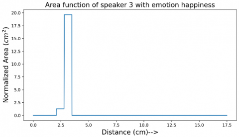
Figure 17. Area function of the vocal tract of speaker 3 for happiness emotion
Figure 18. Area function of the vocal tract of speaker 3 for neutral emotion
Figure 19. Area function of the vocal tract of speaker 3 for anger emotion
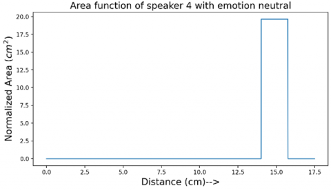
Figure 20. Area function of the vocal tract of speaker 4 for happiness emotion
Figure 21. Area function of the vocal tract of speaker 4 for neutral emotion
Figure 22. Area function of the vocal tract of speaker 4 for anger emotion
Figure 23. Area function of the vocal tract of speaker 5 for happy emotion
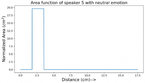
Figure 24. Area function of the vocal tract of speaker 5 for neutral emotion
Figure 25. Area function of the vocal tract of speaker 5 for anger emotion
In this section a brief discussion on the different figures is presented. Figure 5 presents the speech signal of speaker 1 (03 from the Emo-DB) with happy emotion. From the waveform it can be seen that both voiced and unvoiced speech segments are present. Figure 6 presents the STFT of this particular waveform. The frequency seen is 8000 Hz which conforms the Nyquist sampling rate as the sampling frequency is down sampled to 16000 Hz. However, the frequency range of the speech signal can be seen below 4000 Hz, which justifies the straightening of the bend human vocal tract as explained in section 2. A bright spot around 500 Hz and 0.1 s can be noticed in Figure 6. This is the first resonating frequency and zooming in Figure 6 gives the Figure 7. And with this information, the speech signal segment s1(t) is extracted as discussed in section 3. Similarly, another resonating frequency was found near 1000 Hz after zooming in Figure 7 and shown in Figure 8.
Figures 9 and 10 shows the speech segments s1(t) and s2(t) of the speech signal s(t) of the speaker 1 and these are the two solutions considered in obtaining Wronskian of (13).
Figure 11 shows the area function obtained for speaker 1 with the happy emotion. The length of the tract is normalized to 17.5cm and the area of the tract to 19.63cm2 following the discussion in section 3. The area function shown in Figure 11 shows some jump discontinuities. Figures 12-25 show different area functions obtained with the algorithm developed. All these area functions are normalized in length and the area.
It is a known fact that formants do not completely specify the articulation of the tract [5] and also the acoustic to geometry mapping of the human vocal tract is non-unique [7]. Although the area functions obtained for the same emotion of two different speakers cannot be related quantitatively, there are some qualitative similarities. To get a quantitative perspective, number of jump discontinuities of the area functions are counted. The result is summarized in the Table 2. The jump discontinuities for happy and neutral emotion matches for all the speakers at 3 (2 for speaker 6), and 2 jump discontinuities respectively while the anger emotion shows variation at 4 for speaker 1, 3, 4, 5 and 2 for speaker 2 and 3 for speaker 6.
The area function of the speaker 3 with happiness emotion is shown in Figure 17 and with neutral emotion is shown in Figure 18. Also, the area function for the speaker 3 with anger emotion is shown in Figure 19. For speaker 4, the same area functions are shown in Figures 20-22. Same trend can be seen for speaker 5 in Figures 23-25. These results are tabulated in Table 2. The results may be expressed in simple statistics as No. of jump discontinuities for the three emotions can be averaged and expressed as:
Happy=Average 3 with 1 outlier.
Neutral=2 for all the speakers.
Anger=Average 4 with 2 outliers.
The mapping of speech signal to area function of the vocal tract is not unique and it is not surprising to see two different area functions for same emotions. Hence it is difficult to quantify the area functions w.r.t emotions. However, there is some relative information of the tract shapes w.r.t the emotion. In this work an algorithm exploiting the resonance phenomenon is described to estimate the sample (i.e., one out of many possible configuration) area function of a human vocal tract from the speech signals of the speaker. This is based on the simple energy conservation principle. At a certain resonating frequency, a particular shape of the vocal tract would produce a speech signal with a certain emotion if the recording instrument is held near the mouth and the walls of the tract is non-yielding, then energy of the standing wave inside the tract must be equivalent to the energy of the speech signal recorded. At resonance, i.e., for a short period of time, the tract shape would not change substantially and the speech waveform would resemble the standing wave inside the tract. By utilizing this, the area function of the vocal tract is estimated. To get a quantitative perspective of the estimated shapes w.r.t the emotions, the number of discontinuities of the estimated shapes are counted. While the number matches for all the speakers in the case of happy and neutral emotions with 3 (2 for speaker 6) and 2 jump discontinuities respectively, jump discontinuities for the anger emotion varies with 4 for speaker 1, 3, 4, 5 and 2 for speaker 2 and 3 for speaker 6. Although the number of jump discontinuities matches for different speakers with different emotions, for some speakers the jumps are not as big as that of some other speakers. This may be a prospective area for further investigation along with the effect of inserting these area functions in speech synthesis to produce speech with emotions.
|
x |
distance from the glottis. |
|
c |
velocity of sound in air. |
|
t |
time |
|
L |
length of the vocal tract |
|
f |
resonating frequencies |
|
Greek symbols |
|
|
p |
pressure wave. |
|
ω |
eigen frequency. |
|
ρ |
density of air |
Appendix A: Derivation of Webster’s horn equation for a human vocal tract.
Figure 26. Human vocal tract as a non-yielding tube
A non-yielding tube of length L is considered as shown in Figure 26. Let the cross section of the tube is defined as an area function A(x), where x is the distance from the 0 position (glottis). Let us consider an air column inside the tube whose length is bounded between x and x+dx. The air column is not uniform and bounded by the shape of the tube. Let us consider a function ζ(x) that gives the distance from the glottis once the column is activated by the pressure p(x). Using conservation of mass:
$\tilde{p}=\frac{-\rho_0}{A(x)} \frac{\delta}{\delta x}(A(x) \zeta(x))$ (15)
ρ0 is the original density of air in the air column (i. e. before applying pressure), $\tilde{p}$ is the new density of air in the air column after the pressure being applied, A(x) is the area function.
In terms of pressure change:
$\begin{gathered}\tilde{p}=c^2 \tilde{\rho} \\ \tilde{\rho}=\frac{\tilde{p}}{c^2}\end{gathered}$ (16)
where, c is the velocity of sound in air. Putting the value of ρ from 16 in 15, we get:
$\tilde{p}=-c^2 \frac{\rho_0}{A(x)} \frac{\delta}{\delta x}(A(x) \zeta(x))$ (17)
Again, using Newton’s law:
$A(x) \frac{\delta \tilde{p}}{\delta x} \approx \rho_0 A(x) \frac{\delta^2 \zeta(x)}{\delta t^2}$ (18)
Differentiating 18 w.r.t x and putting the value of $\frac{\delta A(x) \zeta(x)}{\delta x}$ from 17 we get:
$\frac{\delta}{\delta x}\left[A(x) \frac{\delta \tilde{p}}{\delta x}\right]=\frac{A(x)}{c^2} \frac{\delta^2 \tilde{p}}{\delta t^2}$ (19)
This is the required Webster’s horn equation. Replacing $\tilde{p}$ of 19 with p(x, t) we get (1).
Appendix B: Abel’s formula
Let s1(x) and s2(x) be two solutions of:
$s^{\prime \prime}(x)+l(x) s^{\prime}(x)+m(x) s(x)=0$ (20)
And let
$W(x)=s_1(x) s_2^{\prime}(x)-s_1^{\prime}(x) s_2(x)$ (21)
Be their Wronskian:
$W^{\prime}(x)=s_1(x) s_2^{\prime \prime}(x)-s_1^{\prime \prime}(x) s_2(x)$ (22)
Since s1(x) and s2(x) are two solutions of 20:
$s_1^{\prime \prime}(x)+l(x) s_1^{\prime}(x)+m(x) s_1(x)=0$ (23)
$s_2^{\prime \prime}(x)+l(x) s_2^{\prime}(x)+m(x) s_2(x)=0$ (24)
Putting the values of $s_1^{\prime \prime}(x)$ and $s_2^{\prime \prime}(x)$ in 22, we get:
$W^{\prime}(x)=-l(x) W(x)$ (25)
Putting $l(x)=\frac{A^{\prime}(x)}{A(x)}$ (comparing 20 with 4), we get:
$\frac{A^{\prime}(x)}{A(x)}=\frac{W^{\prime}(x)}{W(x)}$ or $A(x)=e^{-\int \frac{W^{\prime}(x)}{W(x)} d x}$ (26)
Which is Eq. (13) after considering the limit from 0 (starting point of the tube i.e., glottis) to L (the length of the tube.
[1] Sondhi, M. (1979). Estimation of vocal-tract areas: The need for acoustical measurements. IEEE Transactions on Acoustics, Speech, and Signal Processing, 27(3): 268-273. https://doi.org/10.1109/TASSP.1979.1163240
[2] Wakita, H. (1979). Estimation of vocal-tract shapes from acoustical analysis of the speech wave: The state of the art. IEEE Transactions on Acoustics, Speech, and Signal Processing, 27(3): 281-285. https://doi.org/10.1109/TASSP.1979.1163242
[3] Wakita, H. (1973). Direct estimation of the vocal tract shape by inverse filtering of acoustic speech waveforms. IEEE Transactions on Audio and Electroacoustics, 21(5): 417-427. https://doi.org/10.1109/TAU.1973.1162506
[4] Mitra, V., Nam, H., Espy-Wilson, C.Y., Saltzman, E., Goldstein, L. (2010). Retrieving tract variables from acoustics: A comparison of different machine learning strategies. IEEE Journal of Selected Topics in Signal Processing, 4(6): 1027-1045. https://doi.org/10.1109/JSTSP.2010.2076013
[5] Mermelstein, P. (1967). Determination of the vocal-tract shape from measured formant frequencies. The Journal of the Acoustical Society of America, 41(5): 1283-1294. https://doi.org/10.1121/1.1910470
[6] Sondhi, M.M., Gopinath, B. (1971). Determination of vocal-tract shape from impulse response at the lips. The Journal of the Acoustical Society of America, 49(6B): 1867-1873. https://doi.org/10.1121/1.1912593
[7] Schroeder, M.R. (1967). Determination of the geometry of the human vocal tract by acoustic measurements. The Journal of the Acoustical Society of America, 41(4B): 1002-1010. https://doi.org/10.1121/1.1910429
[8] Schroeter, J., Sondhi, M.M. (1994). Techniques for estimating vocal-tract shapes from the speech signal. IEEE Transactions on Speech and Audio Processing, 2(1): 133-150. https://doi.org/10.1109/89.260356
[9] Mathew, L.R., Manju, S., Gopakumar, K. (2021). Vocal tract parameter estimation and modeling with application in diagnosis of voice disorders. SSRN Electronic Journal. https://dx.doi.org/10.2139/ssrn.3769897
[10] Ogata, K., Kodama, T., Hayakawa, T., Aoki, R. (2019). Inverse estimation of the vocal tract shape based on a vocal tract mapping interface. The Journal of the Acoustical Society of America, 145(4): 1961-1974. https://doi.org/10.1121/1.5095409
[11] Flego, S. (2018). Estimating vocal tract length by minimizing non-uniformity of cross-sectional area. In Proceedings of Meetings on Acoustics 176ASA, 35(1): 060003. https://doi.org/10.1121/2.0001000
[12] Luengo, I., Navas, E., Hernáez, I. (2010). Feature analysis and evaluation for automatic emotion identification in speech. IEEE Transactions on Multimedia, 12(6): 490-501. https://doi.org/10.1109/TMM.2010.2051872
[13] Mongia, P.K., Sharma, R.K. (2014). Estimation and statistical analysis of human voice parameters to investigate the influence of psychological stress and to determine the vocal tract transfer function of an individual. Journal of Computer Networks and Communications, 2014: 290147. https://doi.org/10.1155/2014/290147
[14] Li, Y., Li, J., Akagi, M. (2018). Contributions of the glottal source and vocal tract cues to emotional vowel perception in the valence-arousal space. The Journal of the Acoustical Society of America, 144(2): 908-916. https://doi.org/10.1121/1.5051323
[15] Rabiner, L.R., Schafer, R.W. (1978). Digital processing of speech signals. Prentice-Hall Englewood Cliffs, NJ.
[16] Sondhi, M.M. (1986). Resonances of a bent vocal tract. The Journal of the Acoustical Society of America, 79(4): 1113-1116. https://doi.org/10.1121/1.393383
[17] Webster, A.G. (1977). Acoustical Impedance, and the Theory of Horns and of the Phonograph. Journal of the Audio Engineering Society, 25(1/2): 24-28.
[18] Ross, S.L. (2007). Differential Equations. John Wiley & Sons.
[19] Burkhardt, F., Paeschke, A., Rolfes, M., Sendlmeier, W. F., Weiss, B. (2005). A database of German emotional speech. In Interspeech, 5: 1517-1520.
[20] Lammert, A.C., Narayanan, S.S. (2015). On short-time estimation of vocal tract length from formant frequencies. PloS One, 10(7): e0132193. https://doi.org/10.1371/journal.pone.0132193
[21] Khare, N., Patil, S.B., Kale, S.M., Sumeet, J., Sonali, I., Sumeet, B. (2012). Normal mouth opening in an adult Indian population. Journal of Maxillofacial and Oral Surgery, 11: 309-313. https://doi.org/10.1007/s12663-012-0334-1