Investigating Transfer Learning Performances of Deep Learning Models for Classification of GPR B-Scan Images

Ground Penetrating Radar (GPR) is a fast and efficient way to sense information about subsurface without drilling or digging. The visualization mode of a GPR signal can be done in 1D, 2D or 3D, which are named as A-scan, B-scan, and C-scan, respectively. Buried objects are typically represented as hyperbolas in GPR B-scan images. However, due to the challenging nature of processing such data and its difficult interpretation, automated approaches were needed and developed over time [1]. Although, the number of studies using conventional machine learning techniques were decreased in the past 3-4 years, Support Vector Machines [2], Artificial Neural Networks (ANN) [3, 4], boosting algorithms [5, 6], Hidden Markov Models [7] were utilized for detection and classification tasks on GPR images. With the improvement in computation power of GPUs, deep learning techniques which proved their superiority on image classification started to replace them.

Recently, deep learning techniques have been successfully studied for processing GPR images, including land mine classification [8, 9], classification of soil types [10], subsurface target detection and classification [11-14], object size prediction [15], recognition of tunnel lining elements [16], rebar detection [17, 18], detection of moisture damages [19] and recognition of subgrade defects [20, 21]. All these studies applied deep learning techniques in one of the two ways. The first way is to build a user-defined Convolutional Neural Network (CNN) for the solution of the given problem. Many researchers preferred this way for their specific studies [9, 10, 14, 15, 20, 22, 23]. However, this strategy requires lots of effort and time for deciding an optimal network structure and its optimal hyper parameters. Therefore, some researchers preferred to utilize existing CNN architectures as an alternative and 2^nd way. In this strategy, researchers are required to make a choice of using an existing model with or without its pre-trained weights. Using pre-trained weights obtained from ImageNet is referred as transfer learning. An alternative way is ignoring those weights and train the model from scratch. While the former makes it possible to get faster results, usually higher performance is achieved with the latter if a large dataset is provided. Therefore, seeking a good enough performance with the least effort, which is possible when existing CNN models are used with transfer learning, forms the motivation of this study.

In this paper, a comparative analysis is performed to investigate various existing CNN models using transfer learning. Their classification performances are evaluated on a real bridge deck GPR dataset containing B-scan images. The rest of the paper is organized as follows: Section 2 presents the literature review of the previous studies that utilized existing pre-trained models. In Section 3, a general information about CNNs is given. Section 4 describes the general workflow of the experiments done. In Section 5, information about the dataset, experiments, and the discussion are presented. Finally, Section 6 contains the conclusion.

CNN is a type of deep learning model specifically built for analyzing images. The most notable difference from a conventional feed forward ANN is that CNNs initially include a series of layers which are responsible for feature extraction. It is the design of this part that makes a CNN model superior to others. Typically, it contains some convolutional layers where a set of filters are convolved with the input to obtain feature maps, and some pooling layers for down sampling these maps to reduce the computation. Generally, the output obtained from this part is first flattened and then fed into several fully connected (FC) layers usually designed as a multi-layer Perceptron (MLP) structure. An illustration of such an architecture is given in Figure 1.

1.png

Figure 1. General structure of a CNN

Most CNN configurations use a dropout layer where some neurons are temporarily removed to help overcome the overfitting problem. Another important parameter is the activation function which is responsible for forwarding the amount of information through layers. The most common ones are ReLU, Softmax, tanH and the Sigmoid. Finally, loss functions are used to calculate the predicted error which is optimized in training stage. Cross-Entropy is the most common one, used in classification problems. On the other hand, Euclidean loss function is generally preferred in regression tasks.

Table 1 shows the CNN models used in this study present in Keras API which are publicly available with pre-trained weights [25]. As can be seen from Table 1, the publication year of the CNN models investigated in this study varies from 2015 to 2021. The top-1 accuracy refers to their performance on ImageNet validation dataset. The term depth corresponds to the topological depth of the network, including activation layers, batch normalization layers, etc. The M in number of parameters corresponds to millions.

Table 1. Pretrained CNN models on ImageNet

In experiments, the DECKGPRHv1.0 dataset [27] was used that contains 17,260 GPR B-scan images which are cropped from real bridge deck GPR field data. There are 2 reasons for choosing this dataset. First, it contains cropped images so that a preprocessing is not needed to identify all hyperbolas from a single scan and crop them to feed the proposed model. Possible inaccuracies in this procedure may lead to false alarms in the final classification, thus, these are avoided as well. Second, it is a reliable dataset since it is already used in a past journal study [28]. The dataset contains 8,664 positive and 8,596 negative samples with sizes 50x50 and 48x48, respectively. Some samples from the dataset are given in Figure 3.

3.png

Figure 3. Sample positive (top) and negative (bottom) images

To evaluate the generalization ability of the models 10-fold stratified cross validation was used. The reason of implementing cross-validation using stratified sampling is to maintain the ratio of positive to negative samples in each fold. All models were trained with Adam optimizer where learning rate was set to 10^-3 and the loss function was chosen as Binary Cross Entropy. The training was performed until the loss value converges with a maximum of 100 epochs. To avoid overfitting, early stopping technique was used with a tolerance of 10 epochs. Therefore, if validation loss fails to improve after 10 epochs, the training stops. Among all experiments, the maximum number of epochs reached with this configuration was 41. On the other hand, the shortest training lasted for 17 epochs. A checkpoint mechanism was also included in this configuration. Therefore, when training ends due to early stopping, best weights of the model were loaded back.

Model performances are evaluated by 3 metrics which use the primitives of True Positive (TP), True Negative (TN), False Positive (FP) and False Negative (FN):

- Accuracy: The ratio of the number of correctly classified samples to all samples calculated by Eq. (1).

Accuracy $=\frac{T P+T N}{T P+T N+F P+F N}$           (1)

- Recall: The ratio of the number of correctly classified positive samples to all positive samples calculated by Eq. (2).

$\operatorname{Recall}=\frac{T P}{T P+F N}$          (2)

- Precision: The ratio of the number of correctly classified positive samples to all samples which are predicted as positive, calculated by Eq. (3).

Precision $=\frac{T P}{T P+F P}$          (3)

The results for 10-fold stratified cross validation is given in Table 2. The values are the average of the folds. All experiments were done in Google Collab. Since the GPU assigned for the run varies in each session and model runs were resumed from checkpoints when internet connection fails; a comparison between training times would not be fair, thus, not given. Therefore, models that are too heavy on computation are not considered in this study. However, a general opinion can be formed by examining the inference times of their training on ImageNet. A summary of such information can be found in Keras API where their inference times for both CPU and GPU are presented [25].

Table 2 presents some interesting results. Overall, all models except NasNetMobile achieved 94% or better accuracy even without using data augmentation or training from scratch. The performance of NasNetMobile is not a disappointment though since the classification accuracy is almost 89% with nearly approximately recall and precision. Surprisingly, the best results were obtained by the oldest models ResNet50 and ResNet101 which are introduced in 2015. On the other hand, two variants of the newest model EfficientNetV2 (2021) in Table 1 performed almost identical results (i.e., less than 0.01 accuracy) compared to ResNet variants, thus, missed the first place narrowly. Despite their slightly worse performance, it should be noted that EfficentNet models are the smallest in terms of size except the mobile CNN models (Table 1), and they are usually trained faster while still achieving good results [29]. Comparing its variants, the first versions of EfficentNet (B0 and B4) performed slightly worse compared to V2 versions, as excepted. The next model in top ranking was another old model, Vgg16 (2015), that slightly outperformed EfficientNetB4, however, it fell behind EfficientNetB0.

Table 2. Results of 10-fold stratified cross validation

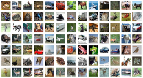
Another surprising result is that the smallest model (i.e., MobileNet) in terms of both depth and number of parameters in Table 1 was able to outclass popular models like DenseNet, Xception and Inception. Considering this together with ResNet’s superiority, it can be concluded that smaller models generally perform better when compared to larger models. This result might not be so surprising after visually examining the GPR B-scan images. Recall that all models in Table 1 were previously trained on RGB images of 1000 categories and their weights, which are obtained after this heavy training, are used to classify GPR images. Some examples of those images are presented in Figure 4 which are taken from CIFAR-100 dataset to give an idea how complicated patterns these RGB images have.

As seen in Figure 3, GPR images have less textural complexity than the images which these models are pre-trained on (Figure 4). Examining the textures in GPR images in Figure 3, it can be derived that those images have circular patterns which are either hyperbola, line, or noise like small granules. The background is generally homogenous or slightly speckled. On the other hand, as seen in Figure 4, RGB images corresponding to real world objects often have much detail due to their variety. Their backgrounds might also include some level of detail if they do not correspond to smooth regions like sky and road. Therefore, instinctively, there is no need to extract complex features to classify GPR B-scan images as opposed to RGB images which contain numerous objects and backgrounds, both usually have detailed textures. Since deeper models with more parameters tend to extract more details compared to smaller models, it is expected that they perform better. However, this is not the case for GPR images, thus, simpler models also have a potential to achieve good results.

4.png

Figure 4. Sample RGB images from CIFAR-100 dataset

In addition to the textural detail, another factor might be the input image size (50x50) which is rather small compared to the input sizes of CNN models that generally have a few hundreds of pixels in height and weight. For instance, ResNet requires a 3-channel input with each having a size of 224x224. Since the level of detail gradually degrades when image size is decreased, number of features to be extracted will also be limited when compared to images with higher resolutions (i.e., sizes). For this reason, smaller models might have gotten the upper hand.

Comparing CNN models with their variants, a similar deduction to the one mentioned about image complexity level can be made. Inspecting the results given in Table 2 together with model sizes (number of parameters and the depth) shown in Table 1, it is seen that many models with the smaller variant outperformed the bigger one, even though the performance difference is rather small. The only exception is ResNet where the larger ResNet101 model achieved almost equal results. The biggest performance difference is observed between MobileNetV2 and MobileNet in which the former obtained more than 4% accuracy. Although, MobileNetV2 has somewhat less parameters compared to MobileNet, it is twice deeper. This also explains the poor performance of NasNetMobile. Although, the number of parameters is not much more than the MobileNet models, NasNetMobile is more than 6 times deeper than MobileNet and more than 3 times deeper than MobileNetV2. Deeper models offer more non-linearity which might be too much for simple cases. Hence, that should have affected those model’s classification ability adversely.