Mingshu Lu | Haiting Liu | Xipeng Yuan*
© 2021 IIETA. This article is published by IIETA and is licensed under the CC BY 4.0 license (http://creativecommons.org/licenses/by/4.0/).
OPEN ACCESS
Infrared thermal imaging can diagnose whether there are faults in electrical equipment during non-stop operation. However, the existing thermal fault diagnosis algorithms fail to consider an important fact: the infrared image of a single band cannot fully reflect the true temperature information of the target. As a result, these algorithms fail to achieve desired effects on target extraction from low-quality infrared images of electrical equipment. To solve the problem, this paper explores the thermal fault diagnosis of electrical equipment in substations based on image fusion. Specifically, a registration and fusion algorithm was proposed for infrared images of electrical equipment in substations; a segmentation and recognition model was established based on mask region-based convolutional neural network (R-CNN) for the said images; the steps of thermal fault diagnosis were detailed for electrical equipment in substations. The proposed model was proved effective through experiments.
infrared thermal imaging, electrical equipment, substation, thermal fault diagnosis
Infrared thermal imaging can diagnose whether there are faults in electrical equipment during non-stop operation [1-8]. In substations, the infrared images of electrical equipment are usually collected by infrared thermal imagers. The collected images need to be checked and judged one by one by experienced engineers. Despite its effectiveness, the manual method is very laborious and slow [9-13]. To prevent major emergency accidents in substations, it is of great significance to study the segmentation of abnormal temperature regions and thermal fault diagnosis based on infrared images of electrical equipment in substations.
Traditional fault detection approaches for electrical equipment have a low accuracy, because infrared images contain interference points, and lack obvious edge features [14-19]. Huang et al. [20] combined residual network (ResNet) with improved watershed algorithm to extract the abnormal areas and fault types of electrical equipment. To accurately segment overheated regions and narrow down the range of fault diagnosis, Fan et al. [21] proposed a novel overheated area detection algorithm of electrical equipment, which adopts Otsu’s method to remove the background, leaving the general areas of electrical equipment. Lin et al. [22] designed an intelligent infrared image fault diagnosis method: the improved deep learning (DL) approach is adopted to detect equipment parts with arbitrary capture angles, and the diagnosis features are extracted from the detection results. Based on fuzzy clustering of fused multi-source data, Qi et al. [23] proposed an infrared image segmentation method, which covers three main steps: producing a saliency map through saliency detection of the infrared image, determining the initial cluster heads, and enhancing the contrast of the original infrared image. For timely diagnosis of thermal anomalies of electrical equipment, Zhao et al. [24] improved the Canny edge detection algorithm to facilitate fault positioning in infrared images of electrical equipment. Specifically, Gaussian filter was replaced with wavelet transform and improved homomorphic filter to improve the flexibility and self-adaptability of Canny edge detection algorithm. The improvement promotes the detection accuracy and adaptability of the original algorithm. Hou [25] relied on adaptive ant colony algorithm to segment the infrared images on electrical equipment, and proved that the algorithm can detect faults in a timely and accurate manner, providing a reliable basis for relevant measures to speed up grid restoration.
For infrared images of electrical equipment in substations, the existing domestic and foreign fault diagnosis methods mainly include the traditional infrared image processing methods, fault diagnosis methods based on expert systems, and methods based on DL. The existing thermal fault diagnosis algorithms fail to consider an important fact: the infrared image of a single band cannot fully reflect the true temperature information of the target. As a result, these algorithms fail to achieve desired effects on target extraction from infrared images of electrical equipment with fuzzy edges. To solve the problem, this paper explores the thermal fault diagnosis of electrical equipment in substations based on image fusion. Section 2 proposes a registration and fusion algorithm for infrared images of electrical equipment in substations; Section 3 derives a segmentation and recognition model based on mask region-based convolutional neural network (R-CNN) for the said images; Section 4 details the steps of thermal fault diagnosis for electrical equipment in substations. The proposed model was proved effective through experiments.
Time changes have a great impact on the infrared imaging effect. Infrared images often contain lots of blind elements and non-uniform fringes, and have a low mean gray value. In general, infrared images can be characterized by solar radiation, gray distribution, and noise features. There are certain differences between infrared images in different bands. Due to hardwire limitation and noises, the fused application of infrared images in different bands concentrates in the imaging scenes of medium and short distances. The infrared images taken in long-distance imaging scenes tend to face large ambiguities and deviations in the texture and edge distribution in different bands, making it difficult to realize pixel-level fusion of multi-band infrared images.
2.1 Feature point detection and registration
Like ordinary visible images, infrared images have two kinds of features: global features like color and texture, and local features that stably characterize local feature points. Global characteristics are susceptible to environmental changes. By contrast, the local features are not easily disturbed by the external environment, and more suitable for image matching. Spots and angular points are the primary local features. In an image, a pixel area can be viewed as a spot, if the pixel differs from the surrounding pixels in gray value. Spots are usually detected by Gaussian Laplacian operator and Hessian matrix. Let W(a, b) be two-dimensional (2D) Gaussian function. Then, Gaussian Laplacian operator can be described as ∇2[W(a, b)]. The spot detection based on Gaussian Laplacian operator firstly convolute the image through Gaussian low-pass filtering, and then convolute the image with Laplacian kernel:
$K(a, b ; \varepsilon)=J(a, b) * W(a, b ; \varepsilon)$ (1)
W(a, b; ε) can be expressed as:
$W(a, b ; \varepsilon)=\frac{1}{2 \pi \varepsilon^{2}} e^{-\frac{a^{2}+b^{2}}{2 \varepsilon^{2}}}$ (2)
Laplacian kernel convolution can be expressed as:
$\nabla^{2} K=\nabla^{2}[W(a, b)] * J(a, b)$ (3)
To sum up, ∇2[W(a, b)] is the Laplacian kernel convolution of W(a, b). On a 2D image, ∇2[W(a, b)] exists as a function with circular symmetry, whose scale can be controlled by ε. This method is almost immune to noise. The spot detection based on Hessian matrix adopts a Hessian matrix (4) and its determinant (5):
$\text { Hessian }=\left[\begin{array}{cc}
K_{a a} & K_{a b} \\
K_{a b} & K_{b b}
\end{array}\right]$ (4)
$\text { det Hessian }=\varepsilon^{4}\left[K_{a a}(a, b, \varepsilon) K_{b b}(a, b, \varepsilon)-K_{a b}^{2}(a, b, \varepsilon)\right]$ (5)
where, det Hessian is the response degree of the image at pixel (a, b) to the matching template. On this basis, it is possible to locate the spot at the scale of ε.
In an image, the intersection of the contours of the object is defined as an angular point, which is another local feature. This paper detects angular points based on Harris algorithm. The gray variation of the image is described by the first-order differential matrix of Harris algorithm. The neighborhood of a pixel is taken as a window to move in all directions. If the first-order differential matrix changes significantly in the neighborhood window of a pixel, then the pixel is as an angular point
2.2 Projection transformation
Owing to the features of infrared images, the image fusion faces limitations in imaging environment, band selection, and hardware requirements. To fuse short-wave and long-wave infrared images, this paper presents a registration algorithm based on the similarity of pixel grayscale distribution, which is suitable for imaging small targets over a long distance. Figure 1 shows the imaging scene.
Figure 1. Small-target imaging model
Let O and P be the target background imaged by cameras 1 and 2, respectively; (a, b) and (s, t) be the coordinates of pixels in O and P, respectively; H be the overlap between O and P; Hab and Hst be the pixel areas corresponding to H in O and P, respectively; F1 and F2 be projection transformation matrices. Based on the principle of camera imaging, the projection relationship can be expressed as:
$H_{a b}=F_{1} H$ (6)
$H_{s t}=F_{2} H$ (7)
The projection transformation relationship between O and P can be derived as:
$H_{a b}=F H_{s t}$ (8)
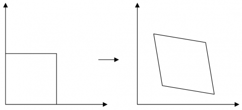
Figure 2. Affine transformation
Similar to the matrix of affine transformation (Figure 2), the form of the transformation matrix F can be given by:
$F=\left[\begin{array}{lll}
f_{11} & f_{21} & f_{13} \\
f_{21} & f_{22} & f_{23} \\
f_{31} & f_{32} & f_{33}
\end{array}\right]$ (9)
where, f11, f12, f21, and f22 are parameters about image changes through scaling and rotation; f13 and f23 are the parameters about image changes through translation; f31 and f32 are the parameters about image changes through projection. Let (a, b) be the coordinates of projection reference point (s, t) projected into the image O through F. Substituting (s, t) into the projection transformation formula (8), we have:
$\left[\begin{array}{l}
a^{\prime} \\
b^{\prime} \\
c^{\prime}
\end{array}\right]=\left[\begin{array}{lll}
f_{11} & f_{21} & f_{13} \\
f_{21} & f_{22} & f_{23} \\
f_{31} & f_{32} & f_{33}
\end{array}\right]\left[\begin{array}{l}
s \\
t \\
1
\end{array}\right]$ (10)
The spatial coordinates (a', b', c') in formula (10) can be adjusted into planar coordinates (a, b) by:
$a=\frac{a^{\prime}}{c^{\prime}}, b=\frac{b^{\prime}}{c^{\prime}}$ (11)
The transformation matrix F can be redefined as:
$F=\left[\begin{array}{lll}
f_{11} & f_{21} & f_{13} \\
f_{21} & f_{22} & f_{23} \\
f_{31} & f_{32} & 1
\end{array}\right]$ (12)
Combining formulas (10)-(12), a homogeneous linear equation system can be obtained for the parameters fT=[f11, f12, f13, f12, f21, f22, f31, f32, 1] of transformation matrix F:
$\left\{\begin{array}{l}
s f_{11}+t f_{12}+f_{13}-s a f_{31}-t a f_{32}-a=0 \\
s f_{21}+t f_{22}+f_{23}-s b f_{31}-t b f_{32}-b=0
\end{array}\right.$ (13)
The above analysis shows that the projection coordinates of the reference point (s, t) can be calculated based on the known values of (s, t) and transformation matrix F.
If at least four pairs of matched (s, t) and (a, b) are known, all the unknown quantities in fT can be solved. Based on formula (13), a homogeneous linear equation system can be established as:
$\left[\begin{array}{ccccccccc}
s_{1} & t_{1} & 1 & 0 & 0 & 0 & -s_{1} a_{1} & -t_{1} a_{1} & -a_{1} \\
0 & 0 & 0 & s_{1} & t_{1} & 1 & -s_{1} b_{1} & -t_{1} b_{1} & -a_{1} \\
& & & & & \vdots & & &
\end{array}\right] f=0$ (14)
Let D be the coefficient matrix of a homogeneous linear equation system. A right singular matrix can be obtained through singular value decomposition (SVD) on D. If no three-point collinearity exists among known projection reference points and projection points, the solution to formula (14) is the last column vector of the right singular matrix.
2.3 Search for the best registration projection point
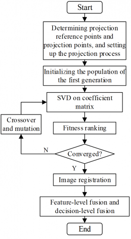
Let MVO and MVP be the edge maps of images O and P, respectively. The traditional registration algorithm combines the extracted O and P feature points to generate multiple pairs of matching points. Unlike the traditional registration algorithm, this paper transforms the registration problem into an optimization problem that searches for the approximate optimal solution on the image plane, with genetic algorithm (GA) as the search method. Figure 3 show the flow of the algorithm.
Figure 3. Flow of registration and optimization problem
As shown in Figure 3, the first step of the GA is to set up the projection process. The projection reference points and projection points in MVO and MVP are binary coded, and taken as chromosomes of the algorithm.
Let (j, l) be the set of coordinates of all points in region Gi; MVO and MVPk be the mean gray values of the two images in region Gi; CO be the correlation coefficient about the similarity between the two images. Then, the fitness of chromosome i can be calculated by the correlation coefficient CO(Gi) between the images with an overlap Gi= MVO ∩MVPi':
$C O\left(G_{i}\right)=\frac{\sum_{j} \sum_{i}\left[M V_{o}(j, l)-\overline{M V_{o}}\right]\left[M V_{P i}^{\prime}(j, l)-\overline{M V}_{P i}^{\prime}\right]}{\sqrt{\left\{\sum_{j} \sum_{l}\left[M V_{o}(j, l)-\overline{M V_{o}}\right]^{2}\right\}\left\{\sum_{j} \sum_{l}\left[M V_{P i}^{\prime}(j, l)-\overline{M V}_{P i}^{\prime}\right]^{2}\right\}}}$ (15)
The correlation coefficient CO falls in the interval of [-1, 1]. If the two images are identical, CO=1.
After initializing the population of the first generation, the population is evolved iteratively to search for the optimal solution. When the iterative process ends, the output coordinates of the optimal projection point are the coded coordinates of the chromosome with the highest fitness.
Image fusion is the last step of the algorithm. Based on the coordinates of the optimal projection point, the optimal transformation matrix can be computed. By projecting P to O, it is possible to obtain P0, i.e., realize image registration. Let G=O∩P0 be the overlap between O and P0. The fusion of equal weight images can be simply expressed as:
$J_{0}=\left\{\begin{array}{l}
O+P_{0},(a, b) \notin G \\
\frac{1}{2}\left(O+P_{0}\right),(a, b) \in G
\end{array}\right.$ (16)
To control image fusion in the feasible range, it is necessary to perform zero-padding in the non-overlapping area (a, b)∉G between the two images with a sufficiently large gray value. In our algorithm, the registration process underpins the fusion process. The accuracy of the registration algorithm ensures the freedom of the fusion process. Considering the features of infrared images in different bands, it is important to design an additional feature- and decision- level fusion algorithm, such that the fused image contains the maximum possible amount of effective information.
During the thermal fault diagnosis on electrical equipment in substations, the collected infrared images include target equipment with overheated parts, normal electrical equipment, and complex backgrounds. The collected infrared images must be segmented accurately and quickly to provide an effective basis for the diagnosis of thermal faults of electrical equipment in substations.
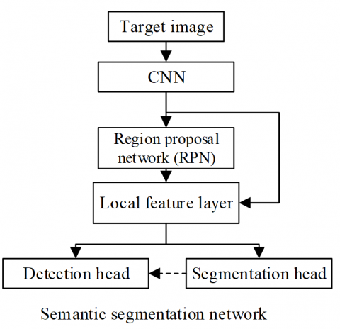
The target equipment in an infrared image can be positioned by two methods: target detection algorithm, and semantic segmentation algorithm. Extended from Faster R-CNN, Mask R-CNN combines the merits of target detection and semantic segmentation to process multiple images simultaneously (Figure 4).
Figure 4. Structure of our CNN model
To enhance the segmentation and recognition capabilities of the model, this paper optimizes the parameter updates of Mask R-CNN based on optimizers. The stochastic gradient descent (SGD) optimizer, and root mean square propagation (RMSProp) optimizers were separately adopted to randomly optimize model parameters.
SDG optimizer trains the network based on randomly selected image samples. The learning unfolds quickly, but tends to fall into local optimum trap. Let ηle be network learning rate; uτ be gradient descent at time τ; Error be the total loss function; Q'τ and Q'τ+1 be the parameters to be optimized at time τ and τ+l, respectively. Then, we have:
$\begin{aligned}
&Q_{t+1}^{\prime}=Q_{\tau}^{\prime}-u_{\tau} \\
&=Q_{\tau}^{\prime}-\eta_{l e} * \frac{\partial E r r o r}{\partial\left(q_{\tau}\right)}
\end{aligned}$ (17)
et hτ be the gradient of the loss function at time τ about the current parameter. Then, the first-order momentum cτ related to the gradient can be described as:
$c_{\tau}=h_{\tau}$ (18)
The second-order momentum Bτ related to the square of the gradient is always equal to 1:
$B_{\tau}=1$ (19)
uτ can be expressed as:
$u_{\tau}=\eta_{l e} * c_{\tau} / \sqrt{B_{\tau}}$ (20)
hτ can be calculated by:
$h_{\tau}=\frac{\partial E r r o r}{\partial\left(q_{\tau}\right)}$ (21)
RMSProp optimizer adds a second-order momentum Eτ to SGD optimizer. Let Vτ be the gradient descent at time τ; Q'’τ and Q’'τ+1 be the parameters to be optimized at time τ and τ+l, respectively. Then, we have:
$\begin{aligned}
&Q_{\tau+1}^{\prime \prime}=Q_{\tau}^{\prime \prime}-V_{\tau} \\
&=Q_{\tau}^{\prime \prime}-\eta_{l e} * \frac{c_{\tau}}{\sqrt{\gamma^{*} E_{\tau-1}+(1-\gamma) h_{\tau}^{2}}}
\end{aligned}$ (22)
The second-order momentum Eτ, which represents the mean over the past period, can be calculated based on the exponential moving average:
$E_{\tau}=\gamma^{*} E_{\tau-1}+(1-\gamma) h_{\tau}^{2}$ (23)
Vτ can be expressed as:
$V_{\tau}=\eta_{l e} * c_{\tau} / \sqrt{E_{\tau}}$ (24)
The network parameters can be adaptively updated by substituting the obtained first-order and second-order momentum into the corresponding parameter update formula above.
Our optimizer inherits the features of SGD and RMSProp optimizers, and combines first- and second-order momentums to correct model deviation. Let Q"'τ and Q"'τ+1 be the parameters to be optimized at time τ and τ+l, respectively. Then, we have:
$\begin{aligned}
&Q_{t+1}^{\prime \prime \prime}=Q_{\tau}^{\prime \prime \prime}-E_{\tau} \\
&=Q_{\tau}-\eta_{l e} * \frac{c_{\tau}}{1-\gamma_{1}^{\tau}} / \sqrt{\frac{E_{\tau}}{1-\gamma_{2}^{\tau}}}
\end{aligned}$ (25)
The first-order momentum cτ can be expressed as:
$c_{\tau}=\gamma_{1} * c_{\tau-1}+\left(1-\gamma_{1}\right) * h_{\tau}$ (26)
The deviation corrected by cτ can be expressed as:
$\tilde{c}_{\tau}=\frac{c_{\tau}}{1-\gamma_{1}^{\tau}}$ (27)
he second-order momentum Eτ can be expressed as:
$E_{\tau}=\gamma_{1} * E_{S-1}+\left(1-\gamma_{2}\right) * h_{\tau}^{2}$ (28)
The deviation corrected by Eτ can be expressed as:
$\tilde{E}_{\tau}=\frac{E_{\tau}}{1-\gamma_{2}^{\tau}}$ (29)
The gradient descent at time τ can be calculated by:
$w_{\tau}=\eta_{l e}{ }^{*} \tilde{c}_{\tau} / \tilde{E}_{\tau}$ (30)
The network parameters can be adaptively updated by substituting the obtained first-order and second-order momentum into the above parameter update formulas.
The thermal fault diagnosis of electrical equipment in substations was completed by temperature difference method. Let ξ be the temperature difference represented by the edges of the different bands of the infrared image; μ1 and μ2 be the temperature rises at overheated points and normal points, respectively; ψ1 and ψ2 be the temperatures at overheated points and normal points, respectively; ψ0 be the ambient temperature. Then, we have:
$\xi=\frac{\mu_{1}-\mu_{2}}{\mu_{1}} \times 100 \%=\frac{\psi_{2}-\psi_{1}}{\psi_{2}-\psi_{0}} \times 100 \%$ (31)
Table 1. Judgement criteria for temperature difference of electrical equipment in substations
|
Equipment name |
Normal |
General fault |
Serious fault |
Critical fault |
|
High-voltage insulating casing |
<0.30 |
≥0.30 |
≥0.90 |
≥0.95 |
|
Suspension insulator |
<0.35 |
≥0.35 |
≥0.80 |
≥0.95 |
|
Supporting insulator |
<0.35 |
≥0.35 |
≥0.80 |
≥0.95 |
|
Sulphur hexafluoride (SF) circuit breaker |
<0.20 |
≥0.20 |
≥0.90 |
≥0.95 |
|
Air circuit breaker |
<0.60 |
≥0.60 |
≥0.90 |
≥0.95 |
|
Connectors and clamps |
<0.40 |
≥0.40 |
≥0.90 |
≥0.95 |
|
Capacitor |
<0.40 |
≥0.40 |
≥0.90 |
≥0.95 |
|
Isolating switch |
<0.40 |
≥0.40 |
≥0.90 |
≥0.95 |
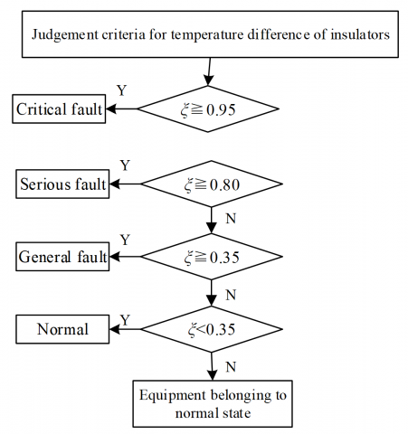
Different judgement criteria should be applied to the temperature difference of various electrical equipment in substations. Table 1 presents the judgment criteria for typical equipment in substations, which help to determine the level of fault. For ordinary insulators, the criteria are as follows: (1) the insulator belongs to the normal state if the temperature difference is within 35%; (2) the insulator has general fault if the temperature difference is from 35% to 80%; (3) the insulator has serious fault if the temperature difference is from 80% to 95%; (4) the insulator has critical fault if the temperature difference is equal to or greater than 95%. Figure 5 shows the flow of thermal fault diagnosis for insulators.
The thermal fault diagnosis algorithm for electrical equipment in substations can be implemented in the following steps:
Step 1. Temperature acquisition
Establish the relationship between the pixel value HF in the colorimetric bar collected by the infrared thermal imager and the device surface temperature ψ reflected by the image:
$\psi=k \cdot H F+\sigma$ (32)
Substitute the peak temperature and the corresponding gray value (HYmax, ψmax), as well as the valley temperature and the corresponding gray value (HYmin, ψmin) into formula (32) to derive the values of k and σ.
Step 2. Preprocessing
Preprocess the infrared image through weighted average graying, median filter denoising, and enhancement through histogram equalization.
Step 3. Segmentation and fusion
Segment and fuse the preprocessed infrared image by the method mentioned in the preceding section, producing the background area Φ1, normal temperature area Φ2, and abnormal temperature area Φ3.
Step 4. Image partitioning
Calculate the mean gray value of areas Φ1, Φ2 and Φ3, separately; identify the area corresponding to the minimum mean gray value as background area 1, that corresponding to the maximum mean gray value as fault area 2, and the remaining area as normal area 0.
Step 5. Mean temperature calculation
Map the gray values obtained in Step 4 according to the results calculated in Step 1, and sort them in descending order: ψ0, ψ1, and ψ2.
Step 6. Fault diagnosis
Judge the fault state of the electrical device against the judgement criteria of temperature difference.
Figure 5. Flow of thermal fault diagnosis for insulators
This paper collects the mean spatial frequency and mean gradient variance of 60 sets of fused images on thermal faults of electrical equipment in substations, and evaluates the fusion effect of infrared images against objective criteria. The results are shown in Table 2.
Table 2. Statistics on fusion effect
|
Image type |
Shortwave image |
Longwave image |
Fused image |
|
Mean spatial frequency |
32.65 |
77.89 |
36.23 |
|
Mean gradient variance |
2.54×10⁵ |
45.78×10⁵ |
9.53×10⁵ |
Under visual enhancement and the low visibility in bad weather, shortwave infrared images make warm targets more recognizable in the cold background. However, the electrical equipment has a low gray value on the infrared images. On the contrary, in the longwave infrared images, the electrical equipment is full of alternating bright and dark areas. This causes inflation to the calculated values of longwave infrared images. As shown in Table 2, many details from shortwave images are added to the fused images, making the latter much clearer.
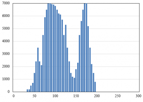
(a) Pre-fusion
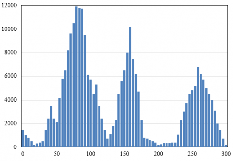
(b) Post-fusion
Figure 6. Gray level histogram effects before and after image fusion
To objectively judge the effect of image registration and fusion, this paper summarizes the frequency of gray values before and after image fusion in each stage, and objectively evaluates the contrast of the fused image. Figure 6 compares the gray level histogram effects before and after image fusion.
Before image registration and fusion, the gray values were concentrated in a small range, a sign of the low contrast and brightness of pre-fusion image. After image fusion, the nonzero values were distributed widely on the histogram, indicating that the fused image has a high contrast and brightness. Therefore, the fused image can better highlight the target, laying a good basis for the thermal fault diagnosis of electrical equipment in substations.
Figure 7. Loss curve of model
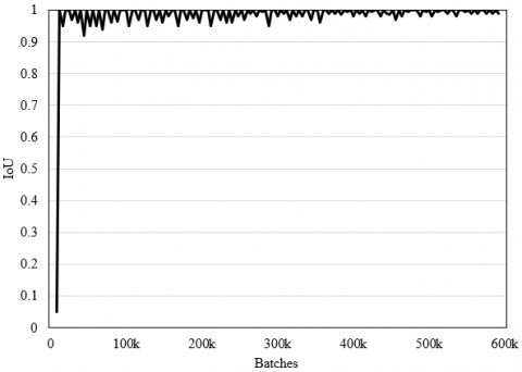
Figure 8. IoU curve of model test
The loss function must ensure that the neural network can pinpoint the abnormal temperature areas, and segment these areas with a high accuracy. Our loss function includes three losses: the loss of classifying the target electrical device, the loss of segmenting the abnormal temperature areas, and the loss of position regression. Figure 7 shows that the total loss of the neural network tended to be stable with the growing number of iterations. The network training started to converge after the 200,000th iteration.
This paper adopts intersection over union (IoU) to measure the quality of fault detection. The closer the label box is to prediction box, the better the detection results. As shown in Figure 8, the rectangular box largely overlapped the fault target, with the growing number of batches.
Taking mean precision as the metric of model performance, Table 3 compares the experimental results and performances of different models. The improved YOLOv3 (you only look once) achieved a mean precision of 92.43%, only 0.32% lower than the image segmentation precision of the traditional Faster R-CNN. However, the improved YOLOv3 far exceeded other one-time regression detectors, such as RetinaNet, SSD300 (single shot detection), in terms of mean precision. Compared with the other models, our model achieved a relatively high mean precision (93.24%) in detecting overheated points on electrical equipment in substations.
The experimental dataset was divided into a training set, a test set, and a verification set by the ratio of 7: 2: 1. The training set has 140 images, the test set has 40 images, and the verification set has 20 images. Some of the images are from the Internet.
Table 3. Experimental results and performances of different models
|
Model type |
Backbone network |
Mean precision (%) |
|
RetinaNet |
ResNet-50 |
78.54 |
|
SSD300 |
ResNet-50 |
82.36 |
|
YOLOv3 |
DarkNet-53 |
86.71 |
|
Improved YOLOv3 |
DarkNet-53 |
92.43 |
|
Faster R-CNN |
VGG16 |
92.75 |
|
Our model |
VGG16 |
93.24 |
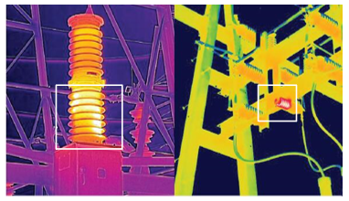
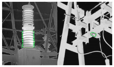
Figure 9 (a) presents the infrared images on the supporting and suspension insulators in a substation under actual working conditions; Figure 9(b) presents the thermal fault diagnosis effect of our algorithm and model. The abnormal temperature areas were roughly indicated by boxes. From the boxes in Figure 9(b), the diagnosis effects on the background area Φ1, normal temperature area Φ2, and abnormal temperature area Φ3 can be further obtained.
The proposed thermal fault diagnosis algorithm was adopted to compute the temperature difference of each electrical device according to the corresponding infrared image. Table 4 records the results on suspension insulator, 380kV high-voltage insulating casing, and supporting insulator of 3kV capacitor bank.
(a)Actual infrared image
(b)Effect of our method
Figure 9. Thermal fault diagnosis results on insulators
Table 4. Temperature differences of different electrical equipment
|
Electrical equipment |
Suspension insulator |
380kV high-voltage insulating casing |
Supporting insulator of 3kV capacitor bank |
|
Φ1 |
13 |
16 |
11 |
|
Φ2 |
24 |
22 |
34 |
|
Φ3 |
49 |
41 |
52 |
|
Temperature difference |
74.3% |
79% |
42% |
As shown in Table 4, the temperature differences of suspension insulator, 380kV high-voltage insulating casing, and supporting insulator of 3kV capacitor bank were 79%, 74.3%, and 42%, respectively. Hence, the thermal faults of the three electrical devices are all general faults, which can be checked and eliminated during shutdown inspection. The experimental results show that the diagnosis results of our thermal fault diagnosis algorithm agree well with the actual faults on the electrical equipment in the substation, indicating that our detection method is feasible and effective.
Based on image fusion, this paper delves into the thermal fault diagnosis of electrical equipment in substations. Firstly, a registration and fusion algorithm was proposed for infrared images of electrical equipment in substations. Then, a Mask R-CNN-based segmentation and recognition model was developed for the said images. The steps of thermal fault diagnosis were then detailed for electrical equipment in substations. Through experiments, the gray level histogram effects before and after image fusion were compared, indicating that the fused image better highlights the target. Then, the proposed neural network was proved feasible by plotting model losses and IoU curves. Further, the superiority of our network was confirmed by comparing the experimental results and performance of our network with several other models. Finally, the thermal fault diagnosis results on insulators were obtained. It was observed that the diagnosis results of our thermal fault diagnosis algorithm agree well with the actual faults on the electrical equipment in the substation.
[1] Zou, H., Huang, F.Z. (2015). An intelligent fault diagnosis method for electrical equipment using infrared images. In 2015 34th Chinese Control Conference (CCC), 6372-6376. https://doi.org/10.1109/ChiCC.2015.7260642
[2] Li, B.S., Xu, X.T., Cui, K.B., Wei, W.L. (2013). Application of infrared imaging technology in fault diagnosis of electrical equipment. In Applied Mechanics and Materials, 401: 974-977. https://doi.org/10.4028/www.scientific.net/AMM.401-403.974
[3] Li, H., Wang, K., Liu, S.J. (2011). Registration method between infrared and visible images of electrical equipment based on gray-scale redundancy and SURF. Power System Protection and Control, 39(11): 111-115.
[4] Men, H., Yu, J., Qin, L. (2011). Segmentation of electric equipment infrared image based on CA and OTSU. Electric Power Automation Equipment, 31(9): 92-95.
[5] Jadin, M.S., Taib, S., Kabir, S., Yusof, M.A.B. (2011). Image processing methods for evaluating infrared thermographic image of electrical equipments. In Proceedings of the Progress in Electromagnetics Research Symposium.
[6] Zhao, Z., Guang, Z., Gao, Q., Wang, K. (2013). Infrared and visible images fusion of electricity transmission equipment using CT-domain hidden Markov tree model. Gaodianya Jishu/High Voltage Engineering, 39(11): 2642-9.
[7] Chen, H. (1994). Applications of infrared imaging system in the defects diagnosis of electric power equipments. Electrics, 24(3): 8-11.
[8] Zhong, H., Lin, X.B., Hu, F., Li, Y.F., Yuan, Z. (2018). Infrared image recognition and development of management system for electrical equipment. In IOP Conference Series: Earth and Environmental Science, 186(5): 012044.
[9] Zhang, C., Yuan, P., Song, C., Yang, Z. (2020). A text recognition method for infrared images of electrical equipment in substations. In 2020 IEEE International Conference on Artificial Intelligence and Computer Applications (ICAICA), pp. 1116-1121. https://doi.org/10.1109/ICAICA50127.2020.9182612
[10] Han, S., Yang, F., Yang, G., Gao, B., Zhang, N., Wang, D. (2020). Electrical equipment identification in infrared images based on ROI-selected CNN method. Electric Power Systems Research, 188: 106534. https://doi.org/10.1016/j.epsr.2020.106534
[11] Yu, Y., Shen, G.T., Ye, C., Li, Y.Q. (2017). Research on image comparison processing technology in electrical equipment infrared thermograph detection. WCCM 2017 - 1st World Congress on Condition Monitoring.
[12] Chen, Y., Dai, J., Mao, X., Liu, Y., Jiang, X. (2017). Image registration between visible and infrared images for electrical equipment inspection robots based on quadrilateral features. In 2017 2nd International Conference on Robotics and Automation Engineering (ICRAE), pp. 126-130. https://doi.org/10.1109/ICRAE.2017.8291366
[13] Yuan, H., Chen, X., Wang, Y., Su, M. (2019). State detection of electrical equipment based on infrared thermal imaging technology. In Chinese Conference on Pattern Recognition and Computer Vision (PRCV), pp. 251-260. https://doi.org/10.1007/978-3-030-31654-9_22
[14] Lin, Y.X., Lin, Y.X. (2018). Reversible data hiding technology for infrared images of electrical equipment based on pixel selection algorithm. Paper Asia, 2018(5): 173-175.
[15] Lin, Y., Qin, J., Zhang, W., Zhang, H., Bai, D., Xu, R. (2018). PCANet based digital recognition for electrical equipment infrared images. In Journal of Physics: Conference Series, 1098(1): 012033.
[16] Zhang, P., Zhang, Y., Cao, H., Liu, S., Yan, D., Yu, Y., Tian, Z. (2018). Outlier-factor-based cluster analysis for infrared image segmentation of electric equipment. In 2018 Chinese Control and Decision Conference (CCDC), pp. 931-936. https://doi.org/10.1109/CCDC.2018.8407263
[17] Dai, J., Liu, Y., He, J., Mao, X., Sheng, G., Jiang, X. (2018). Infrared and visible image fusion of electric equipment using FDST and DC-PCNN. In 2018 Condition Monitoring and Diagnosis (CMD), 1-6. https://doi.org/10.1109/CMD.2018.8535827
[18] Zhou, H., Huang, F. (2017). Multi-target localization for infrared images of electrical equipment based on improved FAsT-Match algorithm. Proceedings of the CSEE, 37(2): 591-599.
[19] Lin, Y., Li, C., Yang, Y., Qin, J., Su, X., Zhang, H., Zhang, W. (2017). Automatic display temperature range adjustment for electrical equipment infrared thermal images. Energy Procedia, 141: 454-459. https://doi.org/10.1016/j.egypro.2017.11.115
[20] Huang, T., Lv, X., Yang, Y., Cheng, M. (2021). Research on fault detection of electrical equipment based on infrared image. In 2021 IEEE 2nd International Conference on Big Data, Artificial Intelligence and Internet of Things Engineering (ICBAIE), pp. 264-268. https://doi.org/10.1109/ICBAIE52039.2021.9389938
[21] Fan, S., Li, T., Liu, Y., Gong, Y., Yu, K. (2020). Infrared image-based detection method of electrical equipment overheating area in substation. In E3S Web of Conferences, 185: 01034. https://doi.org/10.1051/e3sconf/202018501034
[22] Lin, Y., Zhang, W., Zhang, H., Bai, D., Li, J., Xu, R. (2020). An intelligent infrared image fault diagnosis for electrical equipment. In 2020 5th Asia Conference on Power and Electrical Engineering (ACPEE), pp. 1829-1833. https://doi.org/10.1109/ACPEE48638.2020.9136567
[23] Qi, C., Li, Q., Liu, Y., Ni, J., Ma, R., Xu, Z. (2020). Infrared image segmentation based on multi-information fused fuzzy clustering method for electrical equipment. International Journal of Advanced Robotic Systems, 17(2): 1729881420909600. https://orcid.org/0000-0001-5049-7260
[24] Zhao, L., Gao, Q., Yu, X., Song, Y. (2020). Research on improved algorithm of infrared image edge detection for electrical equipment. In 2020 Chinese Automation Congress (CAC), 386-391. https://doi.org/10.1109/CAC51589.2020.9327510
[25] Hou, Y. (2018). Research on infrared image segmentation of electrical equipment based on adaptive ant colony algorithm. Chemical Engineering Transactions, 66: 1303-1308. https://doi.org/10.3303/CET1866218