Qian Zhang | Yi Liu | Lei Liu* | Shuang Lu | Yuxue Feng | Xiao Yu
© 2021 IIETA. This article is published by IIETA and is licensed under the CC BY 4.0 license (http://creativecommons.org/licenses/by/4.0/).
OPEN ACCESS
Currently, tourists tend to plan travel routes and itineraries by searching for relevant information on tourist attractions via the Internet and intelligent terminals. However, it is difficult to achieve good retrieval effect on tourist attraction images with text labels. Based on deep learning, the visual location identification faces such defects as frequent mismatching, high probability of weak matching, and long execution time. To solve these defects, this paper puts forward a novel method for location identification and personalized recommendation of tourist attractions based on image processing. Specifically, the authors detailed the ideas and steps of the location identification algorithm for tourist attractions. The algorithm, grounded on hash retrieval, encompasses two stages: an offline stage, and an online stage. Besides, a personalized recommendation model for tourist attractions based on geographical location and time period. Finally, the proposed algorithm and model were proved accurate and effective through experiments.
image processing, tourist attractions, location identification, personalized recommendation
With the improving level of economy, tourism has become a popular way of leisure. Tourists tend to plan travel routes and itineraries by searching for relevant information on tourist attractions via the Internet and intelligent terminals. Nevertheless, the search results are often not as desired, because they hardly understand the image classification of tourist attractions and have difficulty in organizing the search terms clearly [1-3].
The image retrieval technique of reverse image search can avoid the defects of depicting images with text labels [4, 5]. Therefore, this paper aims to realize location identification and personalized recommendation of tourist attractions. The two tasks were solved based on image processing, for location identification of tourist attractions is usually transformed into an image retrieval problem.
Many scholars have conducted lots of research on image processing of tourist attractions. Based on image processing, some mined the semantics of tourist attractions, some classified the images on tourist attractions, some recommended tourist attractions, and some planned travel routes [6, 7]. Through probabilistic latent semantic analysis (PLSA), Khaliq et al. [8] optimized three semantic-based classification methods for tourist photos, and explored the association between image index semantics, geographical location of tourist attractions, and text labels. Focusing on travel photo libraries with geographic location, Oertel et al. [9] clustered popular landmark attractions based on user interests, and optimized travel routes according to the representative images on landmarks.
Thanks to the progress of online multimedia technology, service providers of smart tourism have paid attention to image retrieval, classification, and positioning. Niu and Qian [10] designed a user-friendly information retrieval system for multiple associated images on tourist attractions. Based on big data analysis and Hadoop distributed platform, Barbeau et al. [11] realized the image matching and retrieval of tourist attraction resource libraries, by optimizing the image quality, storage structure, and geographical location index. Maffra et al. [12] matched local and global features by scale-invariant feature transform (SIFT) / generalized search tree (GiST) for low similarity images, and verified the effectiveness of the feature matching method in positioning tourist attractions on a library of numerous tourist attraction images.
The advancement of artificial intelligence and data mining has promoted the application of depth convolutional neural network (CNN) in image processing. Many researchers have constructed training samples based on online images of tourist attractions to train neural networks, for the purpose of image matching, identification, and positioning [13-16]. Lowry and Milford [17] developed a trained deep neural network not limited to a specific task or dataset, and obtained image feature descriptors like sum pooling of convolutions (SPoC), maximum activation of convolutions (MAC), and regional MAC (rMAC) from the response of convolutional layer; the deep neural network has a good generalization ability and high retrieval accuracy. After collecting the training samples relevant to the target image retrieval task, Sizikova et al. [18] redesigned the deep retrieval architecture of deep neural network, defined the Siamese Loss function, and trained the network again; experimental results show that the trained network is very effective and accurate in the search for tourist attraction images in Oxford5k dataset.
Because the images and geographic coordinates of tourist attraction are easy to obtain, some researches have tried to extract features from tourist attraction images, compute similarities between these images, and identify the tourist attraction locations, with the help of trained deep neural networks; but their algorithms often have a high overhead [19-23]. Doan et al. [24] trained a deep neural network, using tourist attraction images with weak labels of global positioning system (GPS), and obtained the more accurate feature called NetVLAD (where VLAD stands for vector of locally aggregated descriptors); their approach cannot effectively recognize images taken at night, owing to its poor generalization ability and susceptibility to training samples.
When it comes to tourist attraction recommendation, Vysotska and Stachniss [25] constructed a TGSC probabilistic matrix factorization model (PMF), which is aware of geographical location and time, and empirically investigated the influence of popularity, geographical location, and classification over recommendation effect, using the location-based social network (LBSN) dataset. Chen et al. [26] designed a travel route planning model aware of traffic and attraction congestion, after analyzing the tourists’ browsing history on tourist attractions, as well as uncontrollable factors like traffic and weather.
The CNN-based visual location identification of tourist attractions still faces several defects: frequent mismatching, high probability of weak matching, and low computing efficiency. In terms of tourist attraction recommendation, it is highly necessary to improve the efficiency and accuracy of recommendation and tourist preference modeling. Therefore, this paper puts forward a novel method for location identification and personalized recommendation of tourist attractions based on image processing. Section 2 introduces the ideas of the location identification algorithm for tourist attractions, which is based on hash retrieval and composed of an offline stage, and an online stage. Section 3 completes the personalized recommendation of tourist attractions based on geographical location and time period. Finally, the proposed algorithm was proved accurate and effective through experiments.
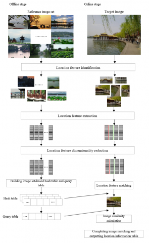
Figure 1. Workflow of the hash retrieval-based location identification algorithm for tourist attractions
To solve the poor matching effect and long identification time of traditional image location identification technology, this section establishes the framework for the two-stage location identification of tourist attraction images based on hash retrieval. The two stages include an offline stage and an online stage. The offline stage mainly creates two tables before system operation: the hash table and the query table for the image location features of the reference image set. The online stage searches for images with similar location features as the target image in the hash table and query table of the reference image set, and constructs a set of candidate images. Figure 1 explains the ideas of the hash retrieval-based location identification algorithm for tourist attractions.
2.1 Offline stage
The offline stage mainly includes four steps: the feature identification, extraction, dimensionality reduction of location features in the reference image set, as well as the construction of the hash table and query table. The edge boxes algorithm, which is based on the edge similarity with the target image, offers a highly adaptive and fast tool to identify targets. It avoids the limitations of advanced model training. Based on the edge boxes algorithm, a location feature extracted from the n-th image in the reference image set can be expressed as:
$LF_{{{I}_{n}}}^{i}(a_{{{I}_{n}}}^{i},b_{{{I}_{n}}}^{i},\Delta a_{{{I}_{n}}}^{i},\Delta b_{{{I}_{n}}}^{i})$. (1)
where, the subscript In means the location feature belong to tourist attraction image In; i is the serial number of the location feature on In; a and b are the coordinates of the upper left corner of the target box of the location feature; Δa and Δb are the width and height of the target box, respectively. Let M be the number of images in the reference image set, and N be the number of location features extracted from each image. Then, In is an integer in [1, M], and I is an integer in [1, N].
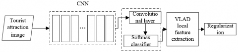
Figure 2. Structure of the CNN
After being identified, the target box of location features needs to be cropped and normalized in size. The CNN extracts the features from the processed box, and outputs the result of LFCIn={LFCIni}. The structure of the CNN is illustrated in Figure 2. The dimensionality reduction of the extracted location features can effectively shorten the execution time of the algorithm. Capable of mapping the center point of an image from the high-dimensional space to a low-dimensional space, Gaussian random projection can control a small Euclidean distance between the two points, without changing the identification and processing effects on the extracted location features. The dimensionality reduction by Gaussian random projection can be described as:
$\left( 1-\varepsilon \right){{\left\| s-r \right\|}^{2}}\le {{\left\| e\cdot s-e\cdot r \right\|}^{2}}\le \left( 1+\varepsilon \right){{\left\| s-r \right\|}^{2}}$ (2)
where, $s$ and $r \in \mathbb{R}^{X}$ are high-dimensional space vectors; $e \in$ $\mathbb{R}^{X \times Y}(Y<<X)$ is the low-dimensional space vector being mapped. After dimensionality reduction, the z-dimensional location features of the reference image set can be expressed as: (LFC΄In1, LFC΄In2, LFC΄In3,…, LFC΄Inz).
During the construction of hash table and query table, the location features after dimensionality reduction should be normalized to the same dimension, such that all of them are distributed on the same high-dimensional sphere:
$\left(\overline{L F_{I_{n}}^{1}}, \ldots, \overline{L F_{I_{n}}^{z}}\right)=\left(\frac{L F_{I_{n}}^{\prime 1}}{\sqrt{\sum_{i=1}^{z}\left(L F_{I_{n}}^{\prime i}\right)^{2}}}, \ldots, \frac{L F_{I_{n}}^{\prime z}}{\sqrt{\sum_{i=1}^{z}\left(L F_{I_{n}}^{\prime i}\right)^{2}}}\right)$ (3)
In Multiple Locality Sensitive Hashing (MutipCpLSH) algorithm, the hash function can map the location features distributed on the same high-dimensional sphere. Within the constructed hash table, every storage unit saves the location features with the same hash code. While the hash table stores location features, the query table stores target box sizes. The two storage functions are of equal importance. In the query table, the index of each target box is the same as that of the corresponding location feature in the hash table. Therefore, the target box corresponding to any location feature can be queried for with the index number.
2.2 Online stage
The retrieval of the target tourist attraction image is completed online. The online stage consists of two phases: preprocessing and matching retrieval. Like the single image processing in offline stage, the preprocessing is also implemented in three steps: feature identification, extraction, and dimensionality reduction. The matching retrieval mainly maps the location features of the target image by MutipCpLSH algorithm, looks up the hash table and query table for the candidate images with the same or similar hash code as the target image, calculates the similarities between two or multiple candidate images, and recommends the candidate image with the highest similarity. Let IIL be the target image. The location feature of the image can be described as:
$LF_{{{I}_{IL}}}^{i}(a_{{{I}_{IL}}}^{i},b_{{{I}_{IL}}}^{i},\Delta a_{{{I}_{IL}}}^{i},\Delta b_{{{I}_{IL}}}^{i})$ (4)
The k-nearest neighbors algorithm (k-NN) algorithm was adopted to look for the candidate images with the same or similar hash code as the target image, owing to its advantages in processing samples that are highly overlapped in classes. Specifically, the k-NN algorithm was executed in each storage unit to calculate the Euclidean distance from the location features of the target image to the K similar location features in each storage unit. The K similar location features constitute a set of candidate location features, where the k-th feature is denoted as δki. The Euclidean distance that expresses the location similarity is denoted as DISki. The set of candidate location features is very likely to contain the global optimal matching location features.
Image similarity calculation mainly targets the shape similarity of target boxes, similarity of location features, and overall similarity of tourist attraction images. The shape similarity of target boxes attempts to eliminate the candidate locations from the set of candidate location features, which are similar in tourist attraction location but different in target box shape. By looking up the tables, the shape of the target box corresponding to the δki-th candidate location feature CLFInj can be obtained. Then, the shape similarity of the target box can be computed by:
$\left\{ \begin{align} & \frac{\left| \Delta a_{{{I}_{IL}}}^{i}-\Delta a_{{{I}_{n}}}^{j} \right|}{\max \left( \Delta a_{{{I}_{IL}}}^{i},\Delta a_{{{I}_{n}}}^{j} \right)}\le \tau \\ & \frac{\left| \Delta b_{{{I}_{IL}}}^{i}-\Delta b_{{{I}_{n}}}^{j} \right|}{\max \left( \Delta b_{{{I}_{IL}}}^{i},\Delta b_{{{I}_{n}}}^{j} \right)}\le \tau \\ \end{align} \right.$ (5)
where, τ=0.25 is the difference in the shape similarity of the target box, that is, the difference in the shape similarity of the target box is controlled under 25%.
Next, it is necessary to compute the similarity between the location feature of the target image and the candidate location features retained through the calculation of the shape similarity of target boxes. The similarity with the δki-th candidate location feature CLFInj can be calculated by:
$S_{\delta_{k}^{i}, C L F_{I_{n}}^{j}}=S_{S} \cdot S_{F}=\exp \left[-\frac{1}{2}\left(\begin{array}{l}\frac{\mid \Delta a_{I_{I L}}^{i}-\Delta a_{I_{n}}^{j}}{\max \left(\Delta a_{I_{I L}}^{i}, \Delta a_{I_{n}}^{j}\right)} \\ +\frac{\left|\Delta b_{I_{I L}}^{i}-\Delta b_{I_{n}}^{j}\right|}{\max \left(\Delta b_{I_{I L}}^{i}, \Delta b_{I_{n}}^{j}\right)}\end{array}\right)\right] \cdot\left[1-\frac{\left(D I S_{k}^{i}\right)^{2}}{2}\right]$ (6)
where, SS and SF are shape similarity and feature similarity. The former is characterized by the exponential function, and the latter by the cosine distance between the two features.
After the calculations of shape similarity of target boxes and location feature similarity, there were at most K remaining candidate images with similar location features as the target image. Then, the candidate images were sorted in descending order of the number of similar location features. Let ICl be the l-th image in the first L images, and l be an integer in [1, L]. The overall similarity of each candidate image and the target image can be calculated by:
$S\left( {{I}_{IL}},I_{C}^{l} \right)=\frac{1}{L}\sum\nolimits_{i,j}{1-S_{\delta _{k}^{i},LC_{I_{C}^{l}}^{j}}^{{}}}$ (7)
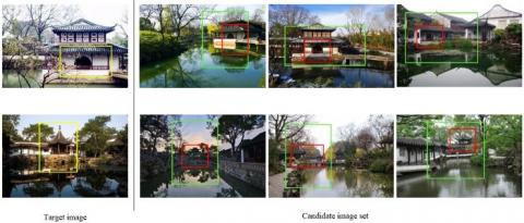
Figure 3. Location feature matching and generation of candidate image set
By a properly set threshold, a group of candidate images with the highest overall similarity was chosen. If the similarity between a candidate image and the target image is greater than the preset threshold, then the candidate image must have been taken at the same geographical location and in the same scene as the target image. In this case, the geographical location of the candidate image could be outputted as the location identification result of the target image. Figure 3 presents the location feature matching effect and the generated set of candidate images.
The probability of a tourist choosing a travel destination or tourist attraction mainly depends on geographical location and time period. The analysis on historical destinations of tourists shows that, if the attractions visited by a tourist are close to each other and densely distributed, it is better to recommend him/her tourist attraction images whose geographical locations are close to the target image and evaluations are general; if the attractions visited by a tourist are far from each other and sparsely distributed, it is better to recommend him/her tourist attraction images whose geographical locations are far from the target image and evaluations are good.
3.1 Geographical location
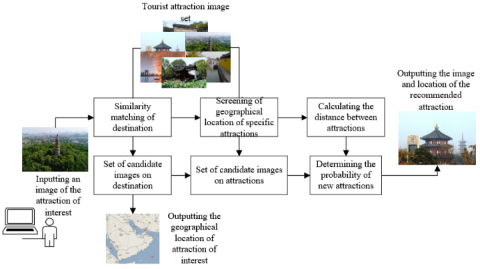
Figure 4. Geographical location-based personalized recommendation algorithm of tourist attractions
Figure 4 explains the ideas of the geographical location-based personalized recommendation algorithm of tourist attractions. The prediction model of historical destinations actually predicts the distance preference from one destination to another. The distance sensitivity of tourists can be modelled by the two methods below:
$D{{S}_{I}}\left( D \right)=\frac{1}{1+D\left( U,V \right)}$ (8)
$D{{S}_{E}}\left( D \right)=\frac{1}{{{e}^{D\left( U,V \right)}}}$ (9)
where, D(U, V) is the distance between destinations U and V. Formula (8) assumes that the tourist sensitivity to the destination distance is negatively correlated with the distance between historical destinations; Formula (9) constructs an exponential function about the distance sensitivity of tourists. Both methods compute the distance between far away destinations with the mean distance. However, neither of them applies to the processing of data on the attractions centering on a particular attraction in the same city.
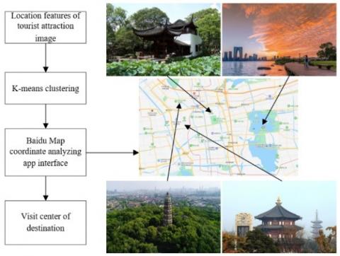
Figure 5. Mining visit center of destination by k-means clustering
After arriving at a destination, a tourist tends to choose attractions around the center of geographical location, or the fixed centers like hotels or special restaurants. If there are many attractions in the city, it is possible to identify the visit center through k-means clustering, compute the distance between each candidate attraction and the center, and make personalized recommendation based on the distance sensitivity of the tourist. Figure 5 explains how to mine the visit center of destination by k-means clustering. Let CA be the set of attractions in the same city; CAT be the set of attractions in the same city that have been visited by tourist T; D(u,v) be the distance between attractions u and v in the same city. Then, the specific modeling process can be described as follows:
Step 1. Compute the distance from each attraction in the destination to the visit center.
Step 2. Model the power law distribution of the tourists’ distance tendencies, convert parameters δ and γ in the solving process, and solve the parameters fitted by converted curve by the least squares method.
Step 3. Derive the probability of choosing a new attraction by the naïve Bayes method:
$\begin{align} & P\left( u|C{{A}_{T}} \right)=\frac{P\left( u\cup C{{A}_{T}} \right)}{P\left( C{{A}_{T}} \right)}=\underset{v\in C{{A}_{T}}}{\mathop{\Pi }}\,P\left[ D\left( u,v \right) \right]=\underset{v\in C{{A}_{T}}}{\mathop{\Pi }}\,\left[ \delta \cdot D{{\left( u,v \right)}^{\gamma }} \right] \\ \end{align}$ (10)
The above geographical location-based recommendation method for destination or attraction assumes that the probability of choosing the destination or attraction at a geographical location has a significant negative correlation with the distance between the location and the current position of the tourist.
3.2 Time period
The popularity of destination or attraction varies between seasons, holidays, and even the hours on the date of travel. The frequency of choosing a destination or an attraction is distributed unevenly from period to period. Museums, science expos, and art galleries, which only open to the public in daytime, are more likely to be chosen during the day, while the entertainment venues are more likely to be selected at night. The popularity of the attractions offering both day and night views is distributed relatively uniformly between different time periods. Let FS-t,U be the probability of choosing destination U in time period t; FT-t,u be the probability of attraction u being visited in time period t; FP(u,t) be the popularity of attraction u in time period t. Under the influence of time period, the popularity of destination or attraction can be calculated by:
$\left\{ \begin{matrix} {{F}_{S-t,U}}=\frac{{{S}_{t}}\left( U \right)}{{{S}_{\Sigma }}\left( U \right)} \\ {{F}_{T-t,u}}=\frac{{{T}_{t}}\left( u \right)}{{{T}_{\Sigma }}\left( u \right)} \\\end{matrix} \right.$ (11)
$F_{P}(u, t)=\frac{1}{\frac{1}{2}\left(\frac{1}{F_{S-t, u}}+\frac{1}{F_{T-t, u}}\right)}=\frac{2+F_{S-t, u} \cdot F_{T-t, u}}{F_{S-t, u}+F_{T-t, u}}$ (12)
where, St(U) is the number of destination U being selected in time period t; Tt(u) is the number of attraction u being visited in time period t; SΣ(U) is the total number of destination U being selected in a year; TΣ(u) is the total number of attraction u being visited in a day. Formula (12) needs to be modified to prevent judging the popularity of the destination or attraction not selected or visited in time period t as zero:
$F_{P}^{*}\left( u,t \right)=\beta \cdot {{F}_{P}}\left( u,t \right)+\left( 1-\beta \right)\cdot {{F}_{P}}\left( u \right)$ (13)
where, FP(u) is the probability of attraction u being visited in a year. Here, each year is divided into 12 periods by month, and every day into 24 periods by hour. Then, the similarity of tourist selection of destination or attraction was modeled by the similarity between time periods. Let ||CVw,t|| be the number of visits of tourist w to destination or attraction in time period t; CSw,t,t΄ be the similarity of the selection of destination or attraction by tourist w between time periods t and t΄. Then, the value of CSw,t,t΄ can be calculated by:
$C{{S}_{w,t,{t}'}}=\frac{\left\| C{{V}_{w,t}} \right\|\cdot \left\| C{{V}_{w,t'}} \right\|}{\sqrt{{{\left\| C{{V}_{w,t}} \right\|}^{2}}\cdot {{\left\| C{{V}_{w,t'}} \right\|}^{2}}}}$ (14)
The similarity between time periods t and t’ can be calculated by:
$C{{S}_{t,{t}'}}=\sum\limits_{w\in W}{\frac{C{{S}_{w,t,{t}'}}}{\left| W \right|}}$ (15)
Let Sw,t,t΄ be an element in the vector of ||CVw,t||. After smoothing by the similarity between time periods, the element can be calculated by:
${{S}_{w,t,u}}=\sum\limits_{{t}'=0}^{T}{\frac{1}{\sum\limits_{{t}''=0}^{T}{C{{S}_{t,{t}''}}}}}\cdot C{{S}_{t,{t}'}}\cdot {{S}_{w,{t}',u}}$ (16)
The similarity between tourists w and o in the selection of destination or attraction u can be calculated by:
$C{{S}_{w,o,t}}=\frac{\sum\limits_{t=0}^{T}{\sum\limits_{u\in \left( {{A}_{w}}\cap {{A}_{o}} \right)}{{{S}_{w,t,u}}\cdot {{S}_{o,t,u}}}}}{\sqrt{\sum\limits_{t=0}^{T}{\sum\limits_{u\in {{A}_{w}}}{{{S}_{w,t,u}}}}*\sum\limits_{t=0}^{T}{\sum\limits_{u\in {{A}_{o}}}{{{S}_{o,t,u}}}}}}$ (17)
The probability that tourist w visits destination or attraction u in the given time period t can be calculated by:
${{P}_{w,t,u}}=\frac{\left( \sum\limits_{v\in U}{C{{S}_{w,o,t}}}\sum\limits_{{{t}'}}^{T}{{{S}_{w,{t}',u}}}\cdot {{S}_{t,{t}'}} \right)}{\sum\limits_{v\in U}{C{{S}_{w,o,t}}}}$ (18)
The experimental data include more than 100,000 images on 84 tourist attractions and their geographical locations. The data were crawled from the online information on domestic tourist attractions. The images were divided into 3 sub-image libraries, and split into a training set and a test set by the ratio of 4:1.
Our algorithm was called to mine the deep features containing the geographical locations of the attractions. Then, hash retrieval was performed to identify the images with high visual similarity of the target image, creating a set of candidate images with similar visual features and geographical locations. The geographical location of the most similar image was outputted, completing the geographical location identification of the input image. Table 1 presents the identification results.
Table 1. An example of geographical location identification
|
Number |
Target image |
Geographical coordinates |
Number |
Target image |
Geographical coordinates |
|
1 |
Jinji Lake N: 31.31 E: 120.70 |
4 |
Zhouzhuang Village N: 31.11 E: 120.85 |
||
|
2 |
Zhuozheng Garden N: 31.32 E: 120.62 |
5 |
Hanshan Temple N: 31.31 E: 120.56 |
||
|
3 |
Huqiu Hill N: 31.33 E: 120.58 |
6 |
Yangcheng Lake N: 31.50 E: 120.72 |
Table 2. Results of geographical location identification
|
Location identification methods |
top-1 |
top-5 |
top-10 |
top-20 |
|
CNN-based method |
10.4 |
20.5 |
40.3 |
76.4 |
|
Dynamic landmark screening-based method |
16.8 |
26.4 |
44.2 |
78.9 |
|
Hash retrieval-based method |
21.1 |
31.8 |
53.9 |
82.1 |
|
Our algorithm |
23.7 |
37.9 |
62.8 |
89.7 |
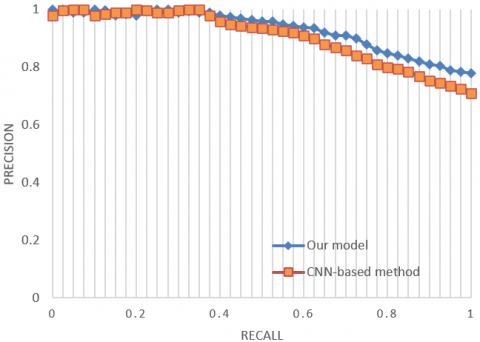
(a)
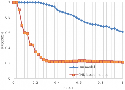
(b)
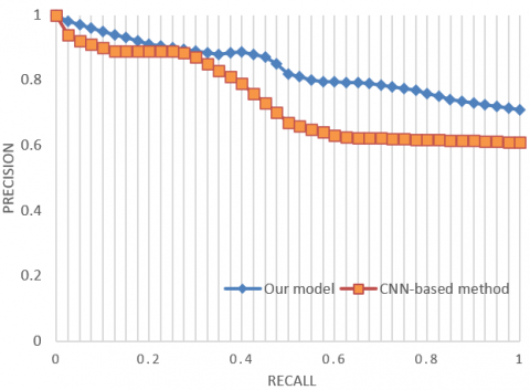
(c)
Figure 6. Precision-recall curves on different image libraries
The candidate images with high similarities were subject to top-N ranking, and the actual location of the attraction images with an error smaller than 50m was determined as the correct geographical location. Table 2 presents the results of geographical location identification.
As shown in Table 2, the recalls of our algorithm for top-1, top-5, top-10, and top-20 rankings were 23.7%, 37.9%, 62.8%, and 89.7%, respectively. Compared with building and intersection images, tourist attraction images cover a large range and exhibit a weak regularity. The proposed geographical location identification method outperformed the methods based on CNN, dynamic landmark screening, or hash retrieval, as evidenced by its high recognition effectiveness.
Figure 6 presents the precision-recall curves of our model (blue) and CNN-based method (orange) on different image libraries. Facing the appearance and visual angle differences between the three image libraries, our model clearly outshined the CNN-based method for geographical location identification. The robustness of our algorithm against different image libraries comes from the inclusion of MutipCpLSH algorithm and edge boxes algorithm into the identification system. The two algorithms promote the global optimal matching of location features, pushing up the identification accuracy of the entire model.
Table 3. Location data on tourist attractions
|
Image number |
Latitude (N) |
Longitude (E) |
|
525733865 |
41.43 |
125.74 |
|
4543856 |
41.51 |
131.55 |
|
31668637 |
42.23 |
127.73 |
|
278558948 |
44.24 |
120.65 |
|
5325769 |
41.59 |
122.71 |
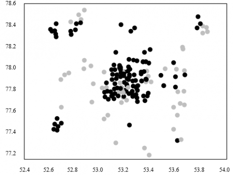
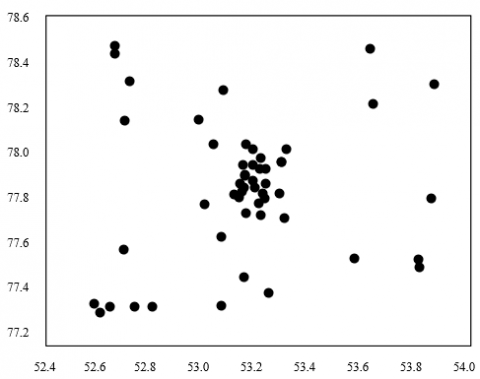
On the recommendation of attractions in the same city, this paper clusters the geographical locations of the attractions (Table 3) in the same city by k-means clustering, and thus obtains the visit center of tourists. Here, a contrastive experiment is designed with different number of cluster heads (K). From the experimental image libraries, 15,000 plus images on ten attractions in a destination were chosen as test samples. Figure 7 shows the clustering results on the geographical locations of the ten attractions at K=50. The left subgraph displays the locations of the attraction images (attraction clusters in different places are given in different shades); the right subgraph presents the 50 cluster heads corresponding to the attraction clusters, i.e., the visit centers of tourists to the destination. The Baidu Map coordinate analyzing app was adopted to obtain the geographical locations of the visit centers, as well as the geographical locations and text illustrations of the nearby attractions.
(a)
(b)
Figure 7. Clustering results on the geographical locations of the ten attractions (K=50)
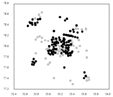
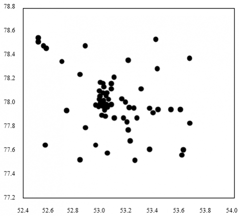
Figure 8 shows the clustering results on the geographical locations of the ten attractions at K=70. Similarly, the left subgraph displays the locations of the attraction images, while the right subgraph presents the 70 cluster heads corresponding to the attraction clusters.
(a)
(b)
Figure 8. Clustering results on the geographical locations of the ten attractions (K=70)
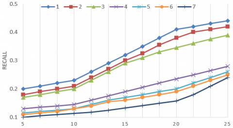
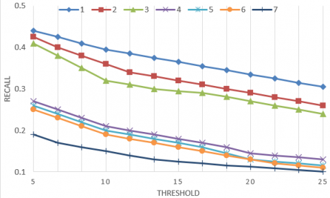
To verify its effectiveness, the proposed personalized tourist attraction recommendation algorithm, which considers both space and time factors, was compared with several tourist attraction recommendation algorithms, some of which are based on matrix decomposition. Figure 9 compares the precision and recall of these algorithms. The contrastive algorithms include: (1) our algorithm; (2) recommendation algorithm based on attraction and tourist similarities; (3) recommendation algorithm based on geographical location of images; (4) recommendation algorithm based on similarity of tourist behaviors; (5) recommendation algorithm based on attraction similarity; (6) recommendation algorithm based on time factor.
(a)
(b)
Figure 9. Precision and recall of different recommendation algorithms for tourist attractions
As shown in Figure 9, algorithm (6) ended up with the worst performance, because it only considers time factors like season or holidays, failing to take account of travel preference of tourists; algorithms (3)-(5) failed to achieve comparable recommendation performance as algorithm (2), for they only consider a single aspect of tourist preference. By contrast, our algorithm boasted the best performance, owing to the comprehensive consideration of various factors (e.g., tourist similarity, attraction similarity, and time period). Our algorithm applies to both nation-wide destination recommendation, and attraction recommendation in the same city. Its application scope is obviously wider than that of the contrastive algorithms.
This paper proposes a novel way to identify the locations and make personalized recommendation of tourist attractions. Firstly, the authors detailed the ideas and steps of the location identification algorithm for tourist attractions based on hash retrieval. Experimental results verify that this algorithm is more effective than CNN-based method, dynamic landmark screening-based method, and simple hash retrieval-based method. Next, a personalized recommendation model was established for tourist attractions based on both geographical location and time period. Comparative experiments revealed that our algorithm boasted the best performance, owing to the comprehensive consideration of various factors (e.g., tourist similarity, attraction similarity, and time period). Our algorithm applies to both nation-wide destination recommendation, and attraction recommendation in the same city. Its application scope is obviously wider than that of the contrastive algorithms.
This paper was supported by the following projects:
(1) Research on color identification system and planning path of traditional villages in central China under the background of rural revitalization strategy, Special Application for Key Research and Development and Promotion of Henan Province, Project No.: 212400410381;
(2) Research on Strategies for Memory Protection and Inheritance of Industrial and Trade Traditional Villages in Henan from the Perspective of Village Culture, Project No.: 2021-ZZJH-453;
(3) Research on Spatial Satisfaction Evaluation and Renewal Protection Strategy for Inheritance of Traditional Village Context in Southern Henan province, Project No.: 2021-ZDJh-422;
(4) Research on the characteristic landscape color recognition system and planning approach of traditional villages in western Henan province, Humanities and Social Sciences research project of Education Department of Henan province in 2020, Project No.: 2020-ZZJH-513;
(5) Research on promoting the characteristic development of Henan cultural industry with social innovation, Subject of Henan social science planning, Project No.: 2018BYS022;
(6) Research on Spatial Feature Improvement design of Traditional Village Landscape in Southern Henan Under Protection Early Warning Strategy, Project No.: 2020-ZZJH-519.
[1] Latif, Y., Doan, A.D., Chin, T.J., Reid, I. (2020). Sprint: Subgraph place recognition for intelligent transportation. In 2020 IEEE International Conference on Robotics and Automation (ICRA), pp. 5408-5414. https://doi.org/10.1109/ICRA40945.2020.9196522
[2] Kim, G., Park, Y.S., Cho, Y., Jeong, J., Kim, A. (2020). Mulran: Multimodal range dataset for urban place recognition. In 2020 IEEE International Conference on Robotics and Automation (ICRA), pp. 6246-6253. https://doi.org/10.1109/ICRA40945.2020.9197298
[3] Leyva-Vallina, M., Strisciuglio, N., Lopez-Antequera, M., Tylecek, R., Blaich, M., Petkov, N. (2019). TB-Places: A Data Set for Visual Place Recognition in Garden Environments. IEEE Access, 7: 52277-52287. https://doi.org/10.1109/ACCESS.2019.2910150
[4] Ferrarini, B., Waheed, M., Waheed, S., Ehsan, S., Milford, M., McDonald-Maier, K.D. (2019). Visual place recognition for aerial robotics: Exploring accuracy-computation trade-off for local image descriptors. In 2019 NASA/ESA Conference on Adaptive Hardware and Systems (AHS), pp. 103-108. https://doi.org/10.1109/AHS.2019.00011
[5] Hausler, S., Jacobson, A., Milford, M. (2019). Multi-process fusion: Visual place recognition using multiple image processing methods. IEEE Robotics and Automation Letters, 4(2): 1924-1931. https://doi.org/10.1109/LRA.2019.2898427
[6] Lopez-Antequera, M., Vallina, M.L., Strisciuglio, N., Petkov, N. (2019). Place and object recognition by CNN-based COSFIRE filters. IEEE Access, 7: 66157-66166. https://doi.org/10.1109/ACCESS.2019.2918267
[7] Kazmi, S.A.M., Mohamed, M.A., Mertsching, B. (2019). Feature-Agnostic Low-Cost Place Recognition for Appearance-Based Mapping. In International Conference on Computer Vision Systems, pp. 49-59. https://doi.org/10.1007/978-3-030-34995-0_5
[8] Khaliq, A., Ehsan, S., Chen, Z., Milford, M., McDonald-Maier, K. (2019). A holistic visual place recognition approach using lightweight cnns for significant viewpoint and appearance changes. IEEE Transactions on Robotics, 36(2): 561-569. https://doi.org/10.1109/TRO.2019.2956352
[9] Oertel, A., Cieslewski, T., Scaramuzza, D. (2020). Augmenting visual place recognition with structural cues. IEEE Robotics and Automation Letters, 5(4): 5534-5541. https://doi.org/10.1109/LRA.2020.3009077
[10] Niu, J., Qian, K. (2020). Robust place recognition based on salient landmarks screening and convolutional neural network features. International Journal of Advanced Robotic Systems, 17(6): 1729881420966966. https://doi.org/10.1177/1729881420966966
[11] Barbeau, M., Garcia-Alfaro, J., Kranakis, E. (2020). Geocaching-Inspired Navigation for Micro Aerial Vehicles with Fallible Place Recognition. In International Conference on Ad-Hoc Networks and Wireless, pp. 55-70. https://doi.org/10.1007/978-3-030-61746-2_5
[12] Maffra, F., Teixeira, L., Chen, Z., Chli, M. (2019). Real-time wide-baseline place recognition using depth completion. IEEE Robotics and Automation Letters, 4(2): 1525-1532. https://doi.org/10.1109/LRA.2019.2895826
[13] Hafez, A.A., Tello, A., Alqaraleh, S. (2019). Visual place recognition by dtw-based sequence alignment. In 2019 27th Signal Processing and Communications Applications Conference (SIU), pp. 1-4. https://doi.org/10.1109/SIU.2019.8806363
[14] Park, C., Chae, H.W., Song, J.B. (2020). Robust Place Recognition Using Illumination-compensated Image-based Deep Convolutional Autoencoder Features. International Journal of Control, Automation and Systems, 18(10): 2699-2707. https://doi.org/10.1007/s12555-019-0891-x
[15] Masatoshi, A., Yuuto, C., Kanji, T., Kentaro, Y. (2015). Leveraging image-based prior in cross-season place recognition. In 2015 IEEE International Conference on Robotics and Automation (ICRA), pp. 5455-5461. https://doi.org/10.1109/ICRA.2015.7139961
[16] Taisho, T., Kanji, T. (2015). Leveraging image based prior for visual place recognition. In 2015 14th IAPR International Conference on Machine Vision Applications (MVA), pp. 194-197. https://doi.org/10.1109/MVA.2015.7153165
[17] Lowry, S., Milford, M.J. (2016). Supervised and unsupervised linear learning techniques for visual place recognition in changing environments. IEEE Transactions on Robotics, 32(3): 600-613. https://doi.org/10.1109/TRO.2016.2545711
[18] Sizikova, E., Singh, V.K., Georgescu, B., Halber, M., Ma, K., Chen, T. (2016). Enhancing place recognition using joint intensity-depth analysis and synthetic data. In European Conference on Computer Vision, pp. 901-908. https://doi.org/10.1007/978-3-319-49409-8_74
[19] Shakeri, M., Zhang, H. (2016). Illumination invariant representation of natural images for visual place recognition. In 2016 IEEE/RSJ International Conference on Intelligent Robots and Systems (IROS), pp. 466-472. https://doi.org/10.1109/IROS.2016.7759095
[20] Li, B.S., Liu, B., Ni, X.S., Huang, P., Pu, L.L. (2020). Research on semantic map generation and location intelligent recognition method for scenic SPOT space perception. The International Archives of Photogrammetry, Remote Sensing and Spatial Information Sciences, 42: 431-435. https://doi.org/10.5194/isprs-archives-XLII-3-W10-431-2020
[21] Benbihi, A., Arravechia, S., Geist, M., Pradalier, C. (2020). Image-based place recognition on bucolic environment across seasons from semantic edge description. In 2020 IEEE International Conference on Robotics and Automation (ICRA), pp. 3032-3038. https://doi.org/10.1109/ICRA40945.2020.9197529
[22] Imbriaco, R., Bondarev, E. (2020). Multiscale convolutional descriptor aggregation for visual place recognition. Electronic Imaging, 2020(10): 313-313. https://doi.org/10.2352/ISSN.2470-1173.2020.10.IPAS-313
[23] Mihankhah, E., Wang, D. (2018). Avoiding to face the challenges of visual place recognition. In Proceedings of SAI Intelligent Systems Conference, pp. 738-749. https://doi.org/10.1007/978-3-030-01054-6_52
[24] Doan, A.D., Latif, Y., Chin, T.J., Liu, Y., Do, T.T., Reid, I. (2019). Scalable place recognition under appearance change for autonomous driving. In Proceedings of the IEEE/CVF International Conference on Computer Vision, pp. 9319-9328.
[25] Vysotska, O., Stachniss, C. (2019). Effective visual place recognition using multi-sequence maps. IEEE Robotics and Automation Letters, 4(2): 1730-1736. https://doi.org/10.1109/LRA.2019.2897160
[26] Chen, Z., Lowry, S., Jacobson, A., Ge, Z., Milford, M. (2015). Distance metric learning for feature-agnostic place recognition. In 2015 IEEE/RSJ International Conference on Intelligent Robots and Systems (IROS), pp. 2556-2563. https://doi.org/10.1109/IROS.2015.7353725