Ahmet Çınar* | Muhammed Yıldırım | Yeşim Eroğlu
© 2021 IIETA. This article is published by IIETA and is licensed under the CC BY 4.0 license (http://creativecommons.org/licenses/by/4.0/).
OPEN ACCESS
Pneumonia is a disease caused by inflammation of the lung tissue that is transmitted by various means, primarily bacteria. Early and accurate diagnosis is important in reducing the morbidity and mortality of the disease. The primary imaging method used for the diagnosis of pneumonia is lung x-ray. While typical imaging findings of pneumonia may be present on lung imaging, nonspecific images may be present. In addition, many health units may not have qualified personnel to perform this procedure or there may be errors in diagnoses made by traditional methods. For this reason, computer systems can be used to prevent error rates that may occur in traditional methods. Many methods have been developed to train data sets. In this article, a new model has been developed based on the layers of the ResNet50. The developed model was compared with the architectures InceptionV3, AlexNet, GoogleNet, ResNet50 and DenseNet201. In the developed model, the maximum accuracy rate was achieved as 97.22%. The model developed was followed by DenseNet201, ResNet50, InceptionV3, GoogleNet and AlexNet, respectively, according to their accuracy. With these developed models, the diagnosis of pneumonia can be made early and accurately, and the treatment management of the patient will be determined quickly.
CNN, deep learning, machine learning, Pneumonia, transfer learning
Pneumonia is an infection of the lungs. It is due to material, purulent, filling the alveoli. There are mainly infective agents such as bacteria, viruses and fungi in its etiology. Pneumonia is an important infectious disease with high morbidity and mortality. Pneumonia is a common reason of death worldwide, especially in child under 5 years. In child under 5 years, 15% of deaths are caused by pneumonia [1]. For this reason, early diagnosis of pneumonia and applying the necessary treatment are of great importance. Imaging methods are extremely important in the diagnosis and management of pneumonia. The most preferred method for diagnosing pneumonia is chest x-ray [2]. According to American Thoracic Society guidelines, if pneumonia is suspected, a posteroanterior chest radiography should be performed. Chest radiography is mainly used to detect newly developing infiltrates or to evaluate response to treatment. In addition, it is involved in evaluating the degree of the disease, detecting complications and determining alternative diagnoses.
The main radiographic findings of pneumonia are segmental or lobar consolidations and interstitial lung disease. Less common radiographic findings are pleural effusion, mediastinal lymphadenopathy, and cavitation. However, the diagnosis may be delayed or misdiagnosed in pneumonia patients due to the non-specific and diverse radiographic findings. It is very important that chest x-ray images are interpreted by experts. Early diagnosis may be delayed in health units where there are not enough specialists. Or there may be a margin of error in conventional diagnoses made by those skilled. Computer-aided applications can be used to prevent these problems [3]. In this way, with early detection, the process is accelerated in non-specialist locations and errors made by conventional methods can be minimized.
Computer-aided technologies have an important place in combating such a widespread and deadly disease [4]. To prevent these fatal diseases, computer-aided systems need to be trained with great numbers of data [5]. The development of CNN layers has provided important gains in the classification of images. In this study, it was aimed to use deep learning models with high performance rates by using large amount of data for the diagnosis of pneumonia [6].
In this paper, the developed hybrid model, Inceptionv3 architecture [7], AlexNet architecture [8], GoogleNet architecture [9], ResNet50 architecture [10] and DenseNet201 architecture [11] are analysed.
In the literature, there are many studies on pneumonia using different models. In their study, Rajaraman et al. reported that they achieved 96.2%-93.6% accuracy in the detection of disease by customizing the Vgg16 model [12]. Saraiva et al. used a database of 5,863 images in total. There are 2 classes, normal and pneumonia. They used the Cnn architecture to train the network. They used Cross verification to verify the network. They stated that they achieved an accuracy rate of 95.30% in their study [13]. Kermany et al. used the Inception V3 model to detect pneumonia. They reported an accuracy rate of 94% to 96.8% [14]. Rajpurkar et al. stated that they have developed a new model called ChexNet consisting of 121 Cnn layers. They stated that were working with 100,000 images of 14 disease types [15]. O’Quinn et al. have described the purpose of their study as developing a CNN network to classify images of pneumonia. In their study, they used a data set consisting of 5,659 images. They stated that classify images with an accuracy rate of 72% by AlexNet Transfer learning method [16]. Varshni et al. reported that they used pre-trained CNN networks to classify x-ray data as normal and abnormal. They stated that obtained the results of their studies statistically [17].
In this paper, 1,341 normal images (non-pneumonia) and 3,875 pneumonia patients were used to detect pneumonia images. The data set used in this section, deep learning and the models used are discussed. Pneumonia data are first classified with the improved model. Then, the classification process was performed using CNN architectures and the results were obtained. The results obtained in Matlab environment [18] are examined in detail in application and results section.
2.1 Dataset
In This data set, which consists of two classes, pneumonia and normal, was taken from Kaggle's website [19]. Training, test and verification folders are available for each class [20, 21]. The data set includes 3,730 pneumonia images and 1,341 normal images. Data set and data numbers are given in Figure 1.
Figure 1. Sample images used in the dataset
2.2 Deep learning
Deep learning is a lower area of the field of machine learning. Especially after 2012, deep learning, which is in a period of pause, became popular again.
It uses many non-linear processing unit layers for deep learning, feature extraction, and conversion. Deep learning architectures consist of several layers that are sequentially ranked. These layers, classified as consecutive, take the output value of the prior layer as the input value.
There are many structures preferred in deep learning. At this study, CNN architectures are examined. CNN networks are the most widely used deep learning networks for classification processes [22].
With the transfer learning models widely used in the deep learning area, pre-trained models are transmitted to the model to be trained. Thus, instead of a model with no knowledge on images, a pre-trained model is utilized.
CNN architectures have shown great development in recent years. Multiple layers are used in CNN networks. In addition, the amount of databases used is increasing day by day. Therefore, GPU-based cards should be preferred over CPU cards used when training networks.
2.3 Structure of system
In In this paper, the ResNet50 architecture that won the ILSVRC imagenet competition in 2015 was used [23] as the base.
Instead of creating a neural network from scratch, ResNet50 model, which is one of the previously created transfer learning methods, is used as the base. Thus, instead of a model with no knowledge on images, the accumulation of a pre-trained model can be utilized. The reason for using ResNet50 is that ResNet50 is successful in biomedical images [24]. It also requires less computational costs by enabling training of data with fewer data sets.
The input layer of the ResNet50 model is arranged to receive data from the data set as 224,224.1. Then the values of the convolution layer following the input layer are updated. In the hybrid model, the last five layers were removed from the 177 layer number, and 10 new layers added to replace those removed layers, increasing the number of layers to 182. The added layers and the final version of the architecture are as in Figure 2.
Figure 2. Proposed architecture
The input, convolution, activation, pooling, fully connected, softmax and classification layers of ResNet50 model are removed and used as the base in the new model. Two different fully connected layers are added on this base. Batch Normalization has been added to normalize each layer of neural networks according to input values and to make the model run more stable and faster. In addition, a Dropout layer is added to prevent the model from memorizing training data. The fully connected layer defined in the output layer classified the data with the help of the Softmax activation function. The added layers are further described.
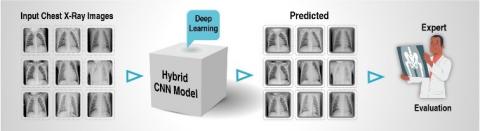
The input, convolution, activation, pooling, fully connected, softmax and classification layers are removed and used as the base in the new model. Two different fully connected layers are added on this base. Batch Normalization has been added to normalize each layer of neural networks according to input values and to make the model run more stable and faster. In addition, a Dropout is added to obstruct the model from memorizing training data. The fully connected defined in the output layer classified the data with the help of the Softmax activation function. The added layers are further described. How the developed hybrid method detects pneumonia from X-ray images is roughly shown in Figure 3.
Figure 3. Interpretation of the outputs by an expert
2.3.1 Input layer
As the name mentions, this layer is the initial layer of the models. High selection of input image size in this layer extends memory requirement, training time and test time. Therefore, the input layer is selected as 224 * 224 * 1 for all architectures.
2.3.2 Activation function
Relu is further known as activation layer. The effect on input data is that it draws negative values to zero. If the network gets a value of zero on the negative axis, it means that the network will run faster. Relu activation function was used in this study. Relu activation function is given in Eq. (1):
$F(x)=\left\{\begin{array}{l}0, x<0 \\ x, x \geq 0\end{array}\right\}$ (1)
The relu layer is more preferred because it has less computational load than other functions [25].
2.3.3 Convolution layer
The convolution layer forms the fundamental of CNN networks. This layer is also called the transformation layer. Convolution is the process of moving a filter over the entire image. The aim of this layer is to produce property maps in convolution layer. the filters selected in this layer are NxN in size.
The convolution of this layer consisting of a series of linear filters is given in Eq. (2):
$\left(h_{k}\right)_{i j}=\left(W_{k} * x\right)_{i j}+b_{i j}$ (2)
where, (i, j) is the index of the pixel point, k is the index of the feature map in this layer, W and b are the weight parameter, x is input data, $\left(h_{k}\right)_{i j}$ is the output value of the feature map [26].
2.3.4 Normalization
In deep learning architectures, normalizing the network enhances the efficiency of the network. The dimensions of the data on other layers may vary. Normalizing the data dimensions from other layers will be healthier. This not only enhance the performance of the architecture, but also scales and plots the input data to a certain range. The Normalization operation is as shown Eqns. (3) and (4):
$X^{k}=\frac{x^{k}-E\left(x^{k}\right)}{\sqrt{\operatorname{Var}\left(x^{k}\right)+\varepsilon}}$ (3)
where, $x^{k}$ define the dimension of the input, $E\left(x^{k}\right)$ define the average of the dimension. $\sqrt{\operatorname{Var}\left(x^{k}\right)+\varepsilon}$ define the standard deviation. $\gamma$ and $\beta$ are set two learnable variables.
$y^{(k)}=\gamma^{k} x^{k}+\beta^{k}$ (4)
2.3.5 Dropout
Deep learning uses large amounts of data when training networks. therefore, the memorization event can occur while the network is being train. Memorization of the network is undesirable. Some nodes need to be disabled to prevent network memorization. Memorization event is blocked after some nodes are disabled. Improve network performance by applying dropout [27]. An example of a network with a dropout operate is as at Figure 4.
Figure 4. Applying dropout
2.3.6 Fully connected layer
This layer, as its name implies, depends on all fields of the prior layer. The data in the prior layer is converted to a one-dimensional matrix structure in the Fully Connected Layer. Class properties of datas can be attained in this layer [28]. The number of fully connected layers used by each architecture may vary.
2.3.7 Pooling layer
The main aims of Pooling are to decrease input size of the data for the subsequent layer. There is no learning process in this layer of the architectures. This layer is mainly used to reduce computational complexity. Average Pooling and Maximum Pooling are commonly used methods. In the pooling layer the filters are chosen in NxN size [29]. As a result of pooling, the size of the resulting image is calculated as in Eq. (5):
$S=w 2 * h 2 * d 2$ (5)
$w 2=\frac{(w 1-f)}{A+1}$ (6)
$h 2=\frac{h 1-f}{A+1}$ (7)
$d 2=d 1$ (8)
$w 1$ = input image size width value
h1 = input image size height value
d1 = input image size depth value
f = filter dimension
A = number of steps
S = Size of produced data
Maximum pooling is used as the pooling layer in the proposed developed hybrid architecture.
2.3.8 Softmax
The Softmax layer takes the values from the prior layer and produces the probabilistic value within the classification process. When classifying the Softmax layer, it produces a value for which class it is closer to. It performs probalistic calculation of the probabilistic value generated in the layer within the deep learning network, revealing the probability value for each class [30].
This layer computes the values for each class as in Eq. (9). These possibilities take values between 0 and 1 to estimate the classes.
$P(y=j \mid x ; W, b)=\frac{\exp ^{X^{T} W_{j}}}{\sum_{j=1}^{n} \exp ^{X^{T} W_{j}}}$ (9)
where, x is main classes W, b a weight vector.
Cross-entropy is used for these procedures. The most commonly used cross-entropy function is given in Eq. (10):
CrossEntropy $=-\sum_{x} P^{\prime}(x) \log P(X)$ (10)
P' denotes the expected output, P denotes the actual output.
2.3.9 Classification
The images are classified in this layer. The result value to be obtained in this layer is as much as the number of groups to be classified. In this study, images are classified as Normal and Pneumonia.
The layers, output dimensions and parameter numbers of the developed architecture are as in Table 1. The improved model consists of a total of 182 layers.
Table 1. Layers of proposed architecture
|
ANALAYSIS RESULT |
|||
|
|
Name |
Activations |
Type |
|
1 |
imageinput |
224x224x1 |
Image Input |
|
2 |
conv_1 |
112x112x64 |
Convolution |
|
172 |
add_16 |
7x7x2048 |
Addition |
|
173 |
relu |
7x7x2048 |
Relu |
|
174 |
conv_2 |
7x7x32 |
Convolution |
|
175 |
batchnorm |
7x7x32 |
Batch Normalization |
|
176 |
dropout |
7x7x32 |
Dropout |
|
177 |
fc_1 |
1x1x2 |
Fully Connected |
|
178 |
activation |
1x1x2 |
Relu |
|
179 |
maxpool |
1x1x2 |
Max Pooling |
|
180 |
fc_2 |
1x1x2 |
Fully Connected |
|
181 |
fc1000_soft |
1x1x2 |
Softmax |
|
182 |
classoutput |
- |
Classification Output |
In addition to the improved model, the network is trained with DenseNet20, ResNet50, AlexNet, InceptionV3 and GoogleNet models and the results are observed.
In this paper, Chest X-Ray images are classified and improved to aid in the diagnosis of pneumonia disease. Hybrid model architecture, Inceptionv3 architecture, AlexNet architecture, GoogleNet architecture, ResNet50 architecture and DenseNet201 architecture models are examined in the paper. The results obtained are compared with the improved model and each other and the necessary inferences are made. The application is carried out in Matlab on a computer with 8GB RAM and i7 processor.
In this paper, the same values are used for obtaining results in all architectures. These values are as in Table 2.
Table 2. The values of the parameters used
|
Solver Name |
Sgdm |
|
MiniBatchSize |
10 |
|
MaxEpochs |
4 |
|
InitialLearnRate |
1.0000e-04 |
|
Shuffle |
every-epoch |
|
ValidationFrequency |
3 |
|
Total Iteration |
1668 |
The confusion matrix is used to describe the performance of the classification model. It allows the visualization of the performance of a model. A confusion matrix is roughly as in Table 3 [31].
Table 3. Confusion matrix
|
|
Normal |
Pneumonia |
|
Normal |
TP |
FP |
|
Pneumonia |
FN |
TN |
Accuracy: It is expressed as the ratio of the correct prediction to the aggregate number of estimates. The accuracy is expressed as in Eq. (11).
Accuracy $=\frac{T P+T N}{T P+T N+F P+F N}$ (11)
Sensitivity: Sensitivity value is obtained by proportioning the total number of correctly estimated data to the aggregate number of correct data [32]. Sensitivity is expressed using Eq. (12).
Sensitivity $=\frac{T P}{T P+E N}$ (12)
Specificity: It is related to the classer's ability to detect negative consequences [33]. Specificity is calculated using Eq. (13).
Specificity $=\frac{T N}{T N+F P}$ (13)
Precision: The Precision value is obtained by dividing the aggregate number of classified positive samples by the estimated aggregate number of positive samples [34]. It is calculated using Eq. (14).
Precision $=\frac{T P}{T P+F P}$ (14)
Recall: Recall is expressed as the rate of the number of correctly classified data to the aggregate number of data. It is calculated using Eq. (15).
Recall $=\frac{T P}{T P+F N}$ (15)
F-measure: It is best if there is some sort of balance between precision and recall in the system. It is the harmonic average of the precision value and recall value. F-measure is calculated using Eq. (16).
$F-$ measure $=\frac{2 * \text { Precision } * \text { Recall }}{\text { Precision }+\text { Recall }}$ (16)
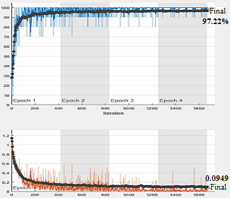
In this paper, the highest accuracy rate was obtained in improved model with 97.22% accuracy rate. This was followed by DenseNet201 with 96.83% accuracy, ResNet50 with 96.35% accuracy, inceptionV3 with 95.35% accuracy, GoogleNet with 94.05% accuracy and AlexNet with 91.07% accuracy.
Improved model's accuracy graphics and loss graphics are as shown in Figure 5.
Figure 5. Improved model’s accuracy and loss graphs
Confusion matrix, sensitivity value, specificity values and F1 Score value of the improved model are as in Table 4.
Table 4. Classification results of the improved model
|
Confusion Matris |
250 |
18 |
|
11 |
763 |
|
|
Accuracy |
97.22 |
|
|
Sensitivity |
95.78 |
|
|
Specificity |
97.69 |
|
|
F-Measure |
94.51 |
|
The accuracy of the improved model is 97.22%. The improved model has a Sensitivity value of 95.78%, Specificity value of 997.69% and F-Measure of 94.51%. 268 classifies 250 of the normal images correctly, while 18 classifies the wrong image. Of the 774 Pneumonia data, 763 were estimated correctly and 11 were incorrectly estimated.
Accuracy and loss graphs obtained in DenseNet201 model in Figure 6, Confusion matrix, sensitivity, specificity and F-Measure values are as in Table 5.
The accuracy rate of the DenseNet201 was 96.83%. The DenseNet201 has a Sensitivity value of 95.36%, Specificity value of 97.31% and F-measure of 93.73%. 268 classifies 247 of the normal images correctly, while 21 classifies the wrong image. Of the 774 diseased data, 762 were estimated correctly and 12 were incorrectly estimated.
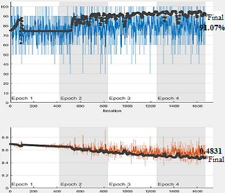
Accuracy and loss graphs obtained in AlexNet in Figure 7, Confusion matrix, sensitivity, specificity and F-measure values are as in Table 6.
The accuracy rate of the AlexNet was 91.07%. The AlexNet has a Sensitivity value of 98.34%, Specificity value of 89.54% and F-measure of 79.28%. 268 classifies 178 of the normal images correctly, while 90 classifies the wrong image. Of the 774 diseased data, 771 were estimated correctly and 3 were incorrectly estimated.
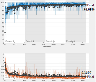
Accuracy and loss graphs obtained in GoogleNet in Figure 8, Confusion matrix, sensitivity, specificity and F-measure values are as in Table 7.
Figure 6. DenseNet201 accuracy and loss graphs
Figure 7. AlexNet accuracy and loss graphs
Table 5. Classification results of the DenseNet201
|
Confusion Matris |
247 |
21 |
|
12 |
762 |
|
|
Accuracy |
96.83 |
|
|
Sensitivity |
95.36 |
|
|
Specificity |
97.31 |
|
|
F-Measure |
93.73 |
|
Table 6. Classification results of the AlexNet
|
Confusion Matris |
178 |
90 |
|
3 |
771 |
|
|
Accuracy |
91.07 |
|
|
Sensitivity |
98.34 |
|
|
Specificity |
89.54 |
|
|
F-Measure |
79.28 |
|
The accuracy rate of the GoogleNet was 94.05%. The GoogleNet has a Sensitivity value of 86.52%, Specificity value of 96.84% and F-measure of 88.72%. 268 classifies 244 of the normal images correctly, while 24 classifies the wrong image. Of the 774 diseased data, 736 were estimated correctly and 38 were incorrectly estimated.
Accuracy and loss graphs obtained in InceptionV3 model in Figure 9, Confusion matrix, sensitivity, specificity and F-measure values are as in Table 8.
Figure 8. GoogleNet accuracy and loss graphs
Table 7. Classification results of the GoogleNet
|
Confusion Matris |
244 |
24 |
|
38 |
736 |
|
|
Accuracy |
94.05 |
|
|
Sensitivity |
86.52 |
|
|
Specificity |
96.84 |
|
|
F-Measure |
88.72 |
|
Figure 9. InceptionV3 accuracy and loss graphs
Table 8. Classification results of the InceptionV3
|
Confusion Matris |
250 |
18 |
|
12 |
762 |
|
|
Accuracy |
95.35 |
|
|
Sensitivity |
95.41 |
|
|
Specificity |
97.69 |
|
|
F-Measure |
94.33 |
|
The accuracy rate of the InceptionV3 was 95.35%. The InceptionV3 has a Sensitivity value of 95.41%, Specificity value of 97.69% and F-measure of 94.33%. 268 classifies 250 of the normal images correctly, while 18 classifies the wrong image. Of the 774 diseased data, 762 were estimated correctly and 12 were incorrectly estimated.
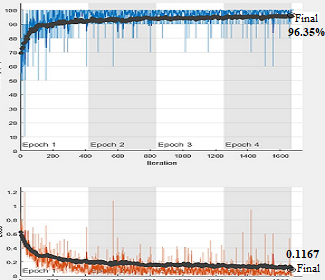
Accuracy and loss graphs showed in ResNet50 in Figure 10, Confusion matrix, sensitivity, specificity and F-measure values are as in Table 9.
Figure 10. ResNet50 accuracy and loss graphs
Table 9. Classification results of the ResNet50
|
Confusion Matris |
249 |
19 |
|
19 |
755 |
|
|
Accuracy |
96.35 |
|
|
Sensitivity |
92.91 |
|
|
Specificity |
97.54 |
|
|
F-Measure |
92.91 |
|
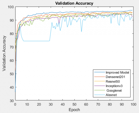
Figure 11. Accuracy graphics of all models
The accuracy rate of the ResNet50 was 96.35%. The ResNet50 has a Sensitivity value of 92.91%, Specificity value of 97.54% and F-measure of 92.91%. 268 classifies 249 of the normal images correctly, while 19 classifies the wrong image. Of the 774 diseased data, 755 were estimated correctly and 19 were incorrectly estimated.
Accuracy graphics and loss graphics of all models are in Figure 11 and Figure 12, Confusion matrix, sensitivity and specificity values are as in Table 10.
In Figure 11, it is seen that the highest accuracy rate is obtained in the hybrid model developed and in Figure 12, the least loss value is obtained in the developed model.
Figure 12. Loss graphics of all models
Table 10. Classification results of the all models
|
|
Accuracy |
Sensitivity |
Specificity |
F-Measure |
|
Improved Model |
97.12 |
95.78 |
97.69 |
94.51 |
|
DenseNet201 |
96.83 |
95.36 |
97.31 |
93.73 |
|
ResNet50 |
96.35 |
92.91 |
97.54 |
92.91 |
|
Inceptionv3 |
95.35 |
95.41 |
97.69 |
94.33 |
|
GoogleNet |
94.05 |
86.52 |
96.84 |
88.72 |
|
AlexNet |
91.07 |
98.34 |
89.54 |
79.28 |
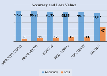
In addition, the accuracy and loss values of all models can be shown in Figure 13. To increase the appearance of loss values in Figure 13, each loss value is multiplied by 100.
Figure 13. Accuracy and values of models
As shown in Table 10 and Figure 13, the highest accuracy was obtained with the developed model with 97.12%. This was followed by DenseNet201 with 96.83%, ResNet50 with 96.35%, InceptionV3 with 95.35%, GoogleNet with 94.05% and AlexNet with 91.07%.
Pneumonia is an inflammation and infection of the lung parenchyma. Pneumonia is the most common cause of death from infection over the age of 60. The annual incidence of pneumonia has been reported at rates ranging from 0.28-1.16%. Its incidence increases in older ages. There are mainly infective agents such as bacteria, viruses and fungi in its etiology. It is divided into three classes as lobar pneumonia, bronchopneumonia, and interstitial pneumonia. In lobar pneumonia, a lobe or segment of the lung is involved and the involved part is in the same pathological stage. There is a widespread involvement in bronchopneumonia, and the infiltration is not limited to a lobe or segment. In interstitial pneumonia, only the interstitial tissue of the lung is involved. Symptoms such as fever, cough, dyspnea and tachypnea are observed in patients with pneumonia. Typical radiological finding of bacterial pneumonia is infiltration involving one or more lobes or segments. In viral pneumonias, unilateral and bilateral reticulogranular infiltrates involving the basal regions and hilar lymphadenopathy are often seen [35]. Pneumonia is one of the most important infectious diseases responsible for serious morbidity and mortality. Radiological imaging methods have an important place in the evaluation of pneumonia patients. Chest x-ray is the most commonly used imaging method in pneumonia due to its easy accessibility and cheapness.
In many studies in the literature, medical data has been classified using deep learning methods. Thanks to the classification obtained with medical data, early diagnosis of many diseases will be easier. Early diagnosis also contributes to the reduction of morbidity and mortality [36].
In this paper, 1,341 normal images (non-pneumonia) and 3,875 pneumonia patients were used to detect pneumonia images. With the improved model in study, an accuracy value of 97.22% was obtained. The proposed hybrid model, 1013 of 1042 test images were correctly classified. It will be possible to determine whether there is pneumonia from the X-ray image given as input to the system with the developed hybrid method.
Table 11. Comparison of the developed model with other deep learning architectures
|
Study |
Year |
Method |
Accuracy |
|
Rajaraman et al. [12] |
2018 |
Vgg16 |
93.6–96.2 |
|
Saraiva et al. [13] |
2019 |
Cnn |
95.3 |
|
Kermany et al. [14] |
2018 |
InceptionV3 |
94–96.8 |
|
Rajpurker et al. [15] |
2017 |
Own model |
95 |
|
O’Quinn et al. [16] |
2019 |
AlexNet |
72.6 |
|
Varshni et al. [17] |
2019 |
ResNet50-SVM |
77.49 |
|
Proposed Study |
2021 |
Developed Hybrid Method |
97.22 |
Similar studies have been made in the literature on the subject. These studies are given in Table 11.
As can be seen in Table 11, the highest accuracy rate has been achieved in the proposed hybrid model. Necessary studies will be carried out to further improve the model in our future works.
In recent years, the use of deep learning methods in clinical and radiology has increased rapidly. This article aims to detect pneumonia in x-ray images using deep learning architectures. Based on some layers of the ResNet50 model, new layers were added to the ResNet50 model and the ResNet50 model was developed. Together with the improved hybrid model, the data was classified with DenseNet201 model, ResNet50 model, InceptionV3 model, GoogleNet model and AlexNet model. The highest accuracy was achieved in the developed model. With the detection of the images of the patients with pneumonia, it will be easier to make inferences about the disease later by the experts. In addition, errors in diagnosis made by conventional methods will be avoided. To train CNN networks, you need to work with big quantity of data. The higher the number of data, the higher the performance of the network. But this brings along the question of time. In order to achieve high performance in Cnn architectures, the amount of data used should be high. Because Cnn architectures work with large amounts of data sets, it takes a long time to train architectures. Gpu cards can be chose to reduce this training time. With high-efficiency cards, the speed problem can be minimized.
[1] Mathur, S., Fuchs, A., Bielicki, J., Anker, J.V.D., Sharland, M. (2018). Antibiotic use for community acquired pneumonia in neonates and children: Who evidence review. Paediatrics and International Child. Health, 38(1): S66-S75. https://doi.org/10.1080/20469047.2017.1409455
[2] Zar, H.J., Andronikou, S., Nicol, M.P. (2017). Advances in the diagnosis of pneumonia in children. BMJ, 358: j2739. https://doi.org/10.1136/bmj.j2739
[3] Çinar, A., Yildirim, M. (2020). Detection of tumors on brain MRI images using the hybrid convolutional neural network architecture. Medical Hypotheses, 139: 109684. https://doi.org/10.1016/j.mehy.2020.109684
[4] Cengıl, E., Çinar, A. (2019). Multiple classification of flower images using transfer learning. In 2019 International Artificial Intelligence and Data Processing Symposium (IDAP), pp. 1-6. https://doi.org/10.1109/IDAP.2019.8875953
[5] Yildirim, M., Çinar, A. (2019). Classification of white blood cells by deep learning methods for diagnosing disease. Revue d'Intelligence Artificielle, 33(5): 335-340. https://doi.org/10.18280/ria.330502
[6] Rai, H.M., Chatterjee, K. (2020). Detection of brain abnormality by a novel Lu-Net deep neural CNN model from MR images. Machine Learning with Applications, 2: 100004. https://doi.org/10.1016/j.mlwa.2020.100004
[7] Szegedy, C., Vanhoucke, V., Ioffe, S., Shlens, J., Wojna, Z. (2016). Rethinking the inception architecture for computer vision. 2016 IEEE Conference on Computer Vision and Pattern Recognition (CVPR), Las Vegas, NV, USA, pp. 2818-2826. https://doi.org/10.1109/CVPR.2016.308
[8] Krizhevsky, A., Sutskever, I., Hinton, G.E. (2012). ImageNet classification with deep convolutional neural networks. In Processing of the 25th International Conference on Neural Information Processing Systems, 1: 1097-1105.
[9] Szegedy, C., Liu, W., Jia, Y.Q., Sermanet, P., Reed, S., Anguelov, D., Erhan, D., Vanhoucke V., Rabinovich, A. (2015). Going deeper with convolutions. In Proceedings of the IEEE Conference on Computer Vision and Pattern Recognition, Boston, MA, USA, pp. 1-9. https://doi.org/10.1109/CVPR.2015.7298594
[10] He, K.M., Zhang, X.Y., Ren, S.Q., Sun, J. (2016). Deep residual learning for image recognition. In Proceedings IEEE Conference on Computer Vision and Pattern Recognition (CVPR), Las Vegas, NV, USA, pp. 770-778. https://doi.org/10.1109/CVPR.2016.90
[11] Huang, G., Liu, Z., Maaten, L.V.D., Weinberger, K.Q. (2017). Densely connected convolutional networks. In Proceedings of the IEEE Conference on Computer Vision and Pattern Recognition, Honolulu, HI, USA, pp. 2261-2269. https://doi.org/10.1109/CVPR.2017.243
[12] Rajaraman, S., Candemir, S., Kim, I., Thoma, G., Antani, S. (2018). Visualization and interpretation of convolutional neural network predictions in detecting pneumonia in pediatric chest radiographs. Applied Sciences, 8(10): 1715. https://doi.org/10.3390/app8101715
[13] Saraiva, A., Ferreira, N., Sousa, L., Carvalho da Costa, N., Sousa, J., Santos, D., Soares, S. (2019). Classification of images of childhood pneumonia using convolutional neural networks. In Proceedings of the 12th International Joint Conference on Biomedical Engineering Systems and Technologies, 2: 112-119. https://doi.org/10.5220/0007404301120119
[14] Kermany, D.S., Goldbaum, M., Cai, W.J., et al. (2018). Identifying medical diagnoses and treatable diseases by image-based deep learning. Cell, 172(5): 1122-1131. https://doi.org/10.1016/j.cell.2018.02.010
[15] Rajpurkar, P., Irvin, J., Zhu, K. et al. (2017). Chexnet: Radiologist-level pneumonia detection on chest x-rays with deep learning. arXiv preprint arXiv:1711.05225.
[16] O’Quinn, W., Haddad, R.J., Moore, D.L. (2019). Pneumonia radiograph diagnosis utilizing deep learning network. 2019 IEEE 2nd International Conference on Electronic Information and Communication Technology (ICEICT), Harbin, China, pp. 763-767, https://doi.org/10.1109/ICEICT.2019.8846438
[17] Varshni, D., Thakral, K., Agarwal, L., Nijhawan, R., Mittal, A. (2019). Pneumonia detection using CNN based feature extraction. 2019 IEEE International Conference on Electrical, Computer and Communication Technologies (ICECCT), Coimbatore, India, pp. 1-7. https://doi.org/10.1109/ICECCT.2019.8869364.
[18] MATLAB. www.mathworks.com/products/matlab.html, accessed on 12 March 2020.
[19] Kaggle, https://www.kaggle.com/paultimothymooney/chest-xray-pneumonia, accessed on 12 March 2020.
[20] Kermany, D., Zhang, K., Goldbaum, M. (2018). Labeled optical coherence tomography (OCT) and Chest X-Ray images for classification. Mendeley Data, 2(2). http://dx.doi.org/10.17632/rscbjbr9sj.2
[21] Pang, L., Lan, Y., Guo, J., Xu, J., Xu, J., Cheng, X. (2017). Deeprank: A new deep architecture for relevance ranking in information retrieval. In Proceedings of the 2017 ACM on Conference on Information and Knowledge Management, pp. 257-266. http://doi.org/10.1145/3132847.3132914
[22] Yildirim, M., Cinar, A. (2020). Classification of Alzheimer's disease MRI images with CNN based hybrid method. Ingénierie des Systèmes d’Information, 25(4): 413-418. https://doi.org/10.18280/isi.250402
[23] Cengıl, E., Çinar, A. (2019). Multiple classification of flower images using transfer learning. In 2019 International Artificial Intelligence and Data Processing Symposium (IDAP), Malatya, Turkey, pp. 1-6. https://doi.org/10.1109/IDAP.2019.8875953
[24] Litjens, G., Kooi, T., Bejnordi, B.E. et al. (2017). A survey on deep learning in medical image analysis. Medical Image Analysis, 42: 60-88. https://doi.org/10.1016/j.media.2017.07.005
[25] Çinar, A., Yildirim, M. (2020). Classification of malaria cell images with deep learning architectures. Ingénierie des Systèmes d’Information, 25(1): 35-39. https://doi.org/10.18280/isi.250105
[26] Indolia, S., Goswami, A.K., Mishra, S.P., Asopa, P. (2018). Conceptual understanding of convolutional neural network-a deep learning approach. Procedia Computer Science, 132: 679-688. https://doi.org/10.1016/j.procs.2018.05.069
[27] Jindal, I., Nokleby, M., Chen, X.W. (2016). Learning deep networks from noisy labels with dropout regularization. In 2016 IEEE 16th International Conference on Data Mining (ICDM), Barcelona, Spain, pp. 967-972. https://doi.org/10.1109/ICDM.2016.0121
[28] Umuroglu, Y., Fraser, N.J., Gambardella, G., Blott, M., Leong, P., Jahre, M., Vissers, K. (2017). Finn: A framework for fast, scalable binarized neural network inference. In Proceedings of the 2017 ACM/SIGDA International Symposium on Field-Programmable Gate Arrays, pp. 65-74. https://doi.org/10.1145/3020078.3021744
[29] Toğaçar, M., Ergen, B., Cömert, Z. (2020). Application of breast cancer diagnosis based on a combination of convolutional neural networks, ridge regression and linear discriminant analysis using invasive breast cancer images processed with autoencoders. Medical hypotheses, 135: 109503. https://doi.org/10.1016/j.mehy.2019.109503
[30] Chawla, A., Lee, B., Fallon, S., Jacob, P. (2018). Host based intrusion detection system with combined CNN/RNN model. In Joint European Conference on Machine Learning and Knowledge Discovery in Databases, pp. 149-158. Springer, Cham. https://doi.org/10.1007/978-3-030-13453-2_12
[31] Swati, S., Kumar, M., Mishra, R.K. (2019). Classification of microarray data using kernel based classifiers. Revue d'Intelligence Artificielle, 33(3): 235-247. https://doi.org/10.18280/ria.330310
[32] Nixon, M., Mahmoodi, S., Zwiggelaar, R. (Eds.). (2018). Medical image understanding and analysis. 22nd Conference, MIUA 2018, Southampton, UK. https://doi.org/10.1007/978-3-319-95921-4
[33] Brinker, T.J., Hekler, A., Enk, A.H., Klode, J., Hauschild, A., Berking, C., Schilling, B., Haferkamp, S., Schadendorf, D., Holland-Letz, T., Utikal, J.S., von Kalle, C. (2019). Deep learning outperformed 136 of 157 dermatologists in a head-to-head dermoscopic melanoma image classification task. European Journal of Cancer, 113: 47-54. https://doi.org/10.1016/j.ejca.2019.04.001
[34] Sofaer, H.R., Hoeting, J.A., Jarnevich, C.S. (2019). The area under the precision‐recall curve as a performance metric for rare binary events. Methods in Ecology and Evolution, 10(4): 565-577. http://doi.org/10.1111/2041-210X.13140
[35] Sattar, S.B.A., Sharma, S. Bacterial Pneumonia. [Updated 2020 Mar 6]. In: StatPearls [Internet]. Treasure Island (FL): StatPearls Publishing.
[36] Yildirim, M., Cinar, A. (2020). A deep learning based hybrid approach for COVID-19 disease detections. Traitement du Signal, 37(3): 461-468. https://doi.org/10.18280/ts.370313