Rabah Hamdini* | Nacira Diffellah | Abderrahmane Namane
© 2019 IIETA. This article is published by IIETA and is licensed under the CC BY 4.0 license (http://creativecommons.org/licenses/by/4.0/).
OPEN ACCESS
Image category recognition is important to access visual information on the level of objects and scene types. In this paper, we propose a new approach for color object recognition using the powerful information provided by the color. This approach is based on the combination of Gray-Edge color constancy, hue components in HSV (hue, saturation, value) color space and cell and bin ideas used in the HOG (Histograms of Gradients) descriptors. The proposed oriented descriptor benefits of the invariance of hues against light intensity change, light intensity shift and light intensity change and shift, and solve its missing of invariance against light color change by using Gray-Edge color constancy. Moreover, the use of cells and bins in this proposed descriptor building boost its invariance the geometric and photo-metric transformation and increases the recognition rate. SVM classifiers (Support Vector Machine) which is a strong classification method known for its flexibility and its power of generalization are used for the training and recognition steps. The proposed method is evaluated on two publicly available datasets including Columbia Object Image Library and The Amsterdam Library of Object Images and obtained a recognition rate of 95.64% and 96.48% – clearly showing the exceptional performance compared to existing methods.
color object recognition, hue, oriented descriptor, SVM, visual information
Recognizing objects from an image is a difficult task in computer vision. Obviously human beings are recognizing objects through vision with high accuracy and little effort, it is still unclear how this perfect performance is achieved. When developing a computer vision model to recognize an object, which rises from challenging theoretical problems, such as how to model the visual appearance and recognize objects. In general object recognition model is framed as image acquisition, prepossessing, feature extraction, and classification [1-6].
A simple and effective recognition scheme is to represent and match images on the basis of color histograms as proposed by Swain and Ballard [7]. The work makes a significant contribution in introducing color for object recognition. However, it has the drawback that when the illumination circumstances are not equal, the object recognition accuracy degrades significantly. This method is extended by Funt and Finlayson [8], based on the re-time theory of Land [9], to make the method illumination independent by indexing on illumination invariant surface descriptors (color ratios) computed from neighboring points. However, it is assumed that neighboring points have the same surface normal. Therefore, the derived illumination-invariant surface descriptors are negatively affected by rapid changes in surface orientation of the object (e.g. the geometry of the object). Healey and Slater [10] and Finlayson et al. [11] use illumination-invariant moments of color distributions for object recognition.
These methods are sensitive to object occlusion and cluttering as the moments are defined as an integral property on the object as one. In global methods, in general, occluded parts will disturb recognition. Slater and Healey [12] circumvent this problem by computing the color features from small object regions instead of the entire object.
To better understand the differences between the detectors, Hoiem et al. [13] provides an extensive analysis of the object detectors and their properties. Their conclusions are that detectors work well for standard object appearances and for common imaging conditions. Evidently, a different construction property of the detectors (e.g. search strategy, functionalities and presentation of the model) influences the robustness of the methods of varying imaging conditions (e.g., unusual views and size of the object, occlusion, clutter). For example, detectors based on the sliding window approach [14] using predefined window sizes and aspect ratios are good for finding likely object positions (positions of the approximate object). However, they are less suited to detect deformable objects with precision. Hoiem et al. [13] shows that these types of detectors usually suffer from poor location errors. On the other hand, a flexible sliding window allows detect deformable objects. The large number of candidates region for detection limits the use of strong classifiers. Therefore, selective search [13] is integrated as pretreatment steps of current state-of the art techniques [15] to reduce the computational complexity of the sliding window based approaches on generating a reduced set of candidates Regions. However, Hosang et al. [16] show that selective research generates candidate regions that are sensitive to changes in scale, illumination and geometric transformations. This result is because selective search is based on segmentation derived from super pixels that are unstable for small distortions of the image.
From the above observations, the choice which colors models to use depends on their robustness against varying illumination across the scene (e.g. multiple light sources with different spectral power distributions) [17], for this in this paper we propose a new recognition method independent of the illumination change based on the combination of Gray-Edge color constancy, hue components in HSV (hue, saturation, value) color space and cell and bin ideas used in the HOG (Histograms of Gradients) descriptors. The proposed feature is effective in recognition of color handmade objects with uniform background.
This paper is organized as follows: In Section 2, we present some old color based feature extraction studies (histogram of oriented gradient (HOG), opponent histogram, hue histogram, SIFT (Scale Invariant Feature Transform) feature and local Image Descriptor from Even Gabor Filter Responses), those methods will be used for a detailed comparison with the proposed methodology. In Section 3 we present our proposed feature and the methodology of building the descriptor. In section 4, Experiments are carried out on Columbia Object Image Library (COIL-100) and The Amsterdam Library of Object Images.
In this section we will present some exciting methods which are opponent histograms, hue histograms of Gever, SIFT features (Scale Invariant Feature Transform) and a local Image Descriptor from Even Gabor Filter Responses. Those classical Color based features will be used for a detailed comparison with the proposed HUE descriptor. But, first we will start by given a definition of light intensity, light intensity shift, light intensity change and shift and light color change.
-Light colors change: According to Kries Model [18], changes in the illumination can be modeled by a diagonal mapping of Von. This diagonal mapping is given as follows:
${{F}^{c}}={{D}^{u,c}}.{{F}^{u}}$ (1)
According to Van de Sande et al. [19], where $F^{u}$ is the image taken under an unknown light source, $F^{c}$ is the same image transformed, so it appears as if it was taken under the reference light (called canonical illuminant), and $D^{u, c}$ is a diagonal matrix which maps colors that are taken under an unknown light source u to their corresponding colors under the canonical illuminant c:
$\left( \begin{matrix} {{R}^{c}} \\ {{G}^{c}} \\ {{B}^{c}} \\\end{matrix} \right)=\left( \begin{matrix} a & 0 & 0 \\ 0 & b & 0 \\ 0 & 0 & c \\\end{matrix} \right)\left( \begin{matrix} {{R}^{u}} \\ {{G}^{u}} \\ {{B}^{u}} \\\end{matrix} \right)$ (2)
R is the red component of images in RGB color space, G is the green one and B represents the bleu component.
-Light intensity change: For Eq. (2), when the image values change by a constant factor in all channels (i.e. a=b=c), this is equal to a light intensity change:
$\left( \begin{matrix} {{R}^{c}} \\ {{G}^{c}} \\ {{B}^{c}} \\\end{matrix} \right)=\left( \begin{matrix} a & 0 & 0 \\ 0 & a & 0 \\ 0 & 0 & a \\\end{matrix} \right)\left( \begin{matrix} {{R}^{u}} \\ {{G}^{u}} \\ {{B}^{u}} \\\end{matrix} \right)$ (3)
Light intensity changes include shadows and lighting geometry changes such as shading. Hence, when a descriptor is invariant to light intensity changes, it is scale-invariant with respect to (light) intensity [19].
-Light intensity shift: An equal shift in images intensity values in all channels, i.e. light intensity shift, where $\left(o_{1}=o_{2}=o_{3}\right)$ and (a=b=c=1) will yield:
$\left( \begin{matrix} {{R}^{c}} \\ {{G}^{c}} \\ {{B}^{c}} \\\end{matrix} \right)=\left( \begin{matrix} {{R}^{u}} \\ {{G}^{u}} \\ {{B}^{u}} \\\end{matrix} \right)+\left( \begin{matrix} {{o}_{1}} \\ {{o}_{1}} \\ {{o}_{1}} \\\end{matrix} \right)$ (4)
Light intensity shifts correspond to object highlights under a white light source and scattering of a white source. When a descriptor is invariant to a light intensity shift, it is shift invariant with respect to light intensity [19].
-Light intensity change and shift: The above classes of changes can be combined to model both intensity changes and shifts:
$\left( \begin{matrix} {{R}^{c}} \\ {{G}^{c}} \\ {{B}^{c}} \\\end{matrix} \right)=\left( \begin{matrix} a & 0 & 0 \\ 0 & a & 0 \\ 0 & 0 & a \\\end{matrix} \right)\left( \begin{matrix} {{R}^{u}} \\ {{G}^{u}} \\ {{B}^{u}} \\\end{matrix} \right)+\left( \begin{matrix} {{o}_{1}} \\ {{o}_{1}} \\ {{o}_{1}} \\\end{matrix} \right)$ (5)
i.e. an image descriptor robust to these changes is scale invariant and shift invariant with respect to light intensity [19].
2.1 HOG (Histogram of Oriented Gradient)
The HOG descriptors were introduced by Dalal and Triggs [20-22]. The main idea of the histogram of oriented gradient is that the local appearance and the shape of the object in an image can be described by the distribution of intensity of the gradients or the direction of contours.
Firstly, the implementation of these descriptors is obtained by dividing the image into small connected areas, called cells, and secondly, in each cell the histogram of the direction of the gradient is calculated. The combination of these histograms represents then the descriptor.
HOG descriptor maintains some key advantages compared to other methods, since the histogram of oriented gradient descriptors operates on localized cells, this method maintains invariance to geometric and photometric transformations, and these changes will only appear in large areas of space.
In the original paper, the HOG features are proposed for pedestrian (human) detection and later many researchers used them to detect some other objects such as cars, dog, cat, etc. Lee et al. [23] show how prediction time can be decreased for car detection. A faster HOG approach for car detection by detecting the shadow region under the cars is proposed by Li and Guo [24]. Hsiao et al. [25] present in detail the implementation of HOG and SVM, for person detection. Bauer et al. [26, 27], and still for person detection, by using an FPGA (Field Programmable Gate Arrays), a CPU (Central Processing Unit), and a GPU (Graphics Processing Unit) in a pipeline architecture, authors present another efficient implementation of the same suite of algorithms.
2.1.1 HOG (Histogram of Oriented Gradient) limitation
As I mentioned before, the Histogram of Oriented Gradient is calculated within a small region of images called cells, we get those cells by dividing the image according to a number of pixels in this image, such as for example, a cell of 8 * 8 pixels or 5 * 5 pixels, in our opinion, for large test image (compared to training images), the HOG is less symmetrical, due to the impact of changing pixels number of the image.
Also, this method is sensitive to illumination condition change, a change in the illumination color and light scattering, shadows and lighting geometry changes such as shading and the highlights under a white light source and scattering of a white source, all this, can operate significantly the recognition rate of this method.
The novelty of our descriptor compared to the HOG is using the stability of hues against the illumination change in the HSV color space and Gray-Edge color constancy to make object colors independent to the light color to make the proposed descriptor robust against illumination conditions change. We also changed the method of choosing cell size to keep the descriptors symmetrical in order to facilitate the classification task and to make our descriptor more invariant to geometric and photometric transformations.
2.2 Opponent histogram
According to Van de Weijer and Schmid [28], channels of the opponent color space are given as:
${{O}_{1}}=\frac{R-G}{\sqrt{2}}$ (6)
${{O}_{2}}=\frac{R+G-2B}{\sqrt{6}}$ (7)
${{O}_{3}}=\frac{R+G+B}{\sqrt{3}}$ (8)
The color information by is represented by the channel $O_1$ and $O_2$ and the intensity information is represented by $O_3$. The opponent angle $\operatorname{ang}_{x}^{o}$ in opponents color space is supposed to be specular invariant [28]. This opponent angle is defined as:
$ang_{x}^{O}=arctag\left( \frac{{{O}_{1x}}}{{{O}_{2x}}} \right)$ (9)
where, $O_{1 x}$ denotes the first order derivative of $O_1$, etc. Authors in [28] applied an error analysis to the opponent angle. Here, $\partial a n g_{x}^{O}$ is defined as the weight of the opponent angle:
$\partial ang_{x}^{O}=\frac{1}{\sqrt{O_{1x}^{2}+O_{2x}^{2}}}$ (10)
The opponent histogram is quantized to 36 bins. For more details about opponent descriptors the reader will be able to refer to [28, 29].
2.2.1 Opponent histogram limitation
According to Van de Sande et al. [19], opponent histograms in not invariant to light intensity change, light intensity shift, light intensity change and shift and light color change. So this feature is not invariant to change in shadows and lighting geometry changes such as shading, object highlights under a white light source and scattering of a white source and to a change in the illumination color and light scattering. Moreover, this descriptor is not invariant to geometric and photometric transformation.
The proposed hue descriptor solves those drawbacks by the use of the hue which is invariant to light intensity change (change in shadows and lighting geometry changes such as shading), light intensity shift (objects highlights under a white light source and scattering of a white source) and light intensity change and shift(combinations of the above two conditions), and also the Gray-Edge color constancy to solve the problem of missing invariance to the light color change(change in the illumination color and light scattering). Moreover, cells and bin ideas used in the proposed hue descriptor solve the lack of invariance to geometric and photometric transformation.
2.3 Hue histograms
The hue becomes unstable near the Gray axis in the HSV color space. To this end, Van de Weijer et al. [29] apply an error propagation analysis to the hue transformation. The analysis shows that the certainty of the hue is inversely proportional to the saturation. Therefore, the hue histogram is made more robust by weighing each sample of the hue by its saturation. The H color model is scale-invariant and shift-invariant with respect to light intensity.
Hue and saturation of HSV color space can be computed from opponent colors [28]:
$hue=\arctan \left( \frac{{{O}_{1}}}{{{O}_{2}}} \right)=\arctan \left( \frac{\sqrt{3}\left( R-G \right)}{R+G-2B} \right)$ (11)
$\begin{align} & saturation=\sqrt{O_{1}^{2}+O_{1}^{2}} \\ & \,\,\,\,\,\,\,\,\,\,\,\,\,\,\,\,\,\,\,\,\,\,\,=\sqrt{\frac{2}{3}\left( {{R}^{2}}+{{G}^{2}}+{{B}^{2}}-RG-RB+GB \right)} \\ \end{align}$ (12)
where, $O_1$ and $O_2$ are two components from opponent’s color space cites in Eq. (6) and equation Eq. (7), respectively.
Same to the opponent histogram, hue histogram is quantized to 36 bins. For more details about opponent descriptors the reader will be able to refer to [28, 29].
In last few years, and because of the invariance of hue to the illumination change, many authors propose descriptors built using hue. In our experiment we will use the hue histogram cited by Van de Sande et al. [19].
2.3.1 Hue histogram limitation
According to Van de Sande et al. [19], hue histograms is not invariant to light color changes, so the recognition rate will be affected by a change in the illumination color and light scattering. Furthermore, its building strategy is not effective in large scales, so the recognition system will not be invariance to geometric and photometric transformation. The novelty of the proposed hue descriptor compared to this hue histograms is the use Gray-Edge color constancy to make the descriptor invariant to the light color changes, and also changing the methodology of building the descriptor by using cell and bin ideas, this new methodology of buildings make the descriptor invariant to geometric and photo-metric transformation.
2.4 SIFT features
Scale Invariant Feature Transform (SIFT) is originally presented in 2004 by Lowe [30] as a strength descriptor for object detection and recognition. The SIFT features are computed in four steps. The first one is to determine local key points, those points are important and stable for given images. Then features are extracted from each key point that explains the local image region samples, which are related to its scale space coordinate image. In the second step, weak features are removed by a specific threshold value. In the third step, orientations are assigned to each key point based on local image gradient directions. Finally, the 1*128 dimensional feature vector is extracted, and bi-linear interpolation is performed to improve the robustness of features. The above theory is defined through equations Eq. (13), Eq. (14) and Eq. (15).
$\xi \left( \mu ,\nu ,\sigma \right)={{\psi }_{G}}\left( \mu ,\nu ,\sigma \right)\otimes {{S}_{final}}\left( {{X}_{i}} \right)$ (13)
${{\psi }_{G}}\left( \mu ,\nu ,\sigma \right)=\frac{1}{2\pi {{\sigma }^{2}}}{{e}^{-\frac{1}{2}\left( \frac{{{\mu }^{2}}+{{\nu }^{2}}}{2{{\sigma }^{2}}} \right)}}$ (14)
$\begin{align} & D\left( \mu ,\nu ,\sigma \right)=\left( {{\psi }_{G}}\left( \mu ,\nu ,k\sigma \right)-{{\psi }_{G}}\left( \mu ,\nu ,\sigma \right) \right) \\ & \quad \quad \quad \quad \,\,\,\,\,\otimes {{S}_{final}}\left( Xi \right)=\xi \left( \mu ,\nu ,k\sigma \right)-\xi \left( \mu ,\nu ,\sigma \right) \\ \end{align}$ (15)
where, $\xi(\mu, \nu, \sigma)$ is scale space of an image, $\psi(\mu, v, k \sigma)$ denotes the variable-scale Gaussian, k is a multiplicative factor D(μ,ν,σ) denotes the difference of Gaussian convolved with a segmented image. For more details about SIFT feature, the reader will be able to refer to the paper [30].
2.4.1 SIFT features limitation
The drawback of SIFT feature is that it is mathematically complicated and computationally heavy. SIFT is based on the Histogram of Gradients. That is, the gradients of each Pixel in the patch need to be computed and these computations cost time. Moreover SIFT feature is not effective for low-powered devices. Moreover the SIFT descriptor is not invariant to light color changes, because the intensity channel is a combination of R, G and B channels [19]. The proposed hue descriptor solves this drawback by using color which improve the recognition rate. Furthermore, its construction method is less complicated, then the calculation time will be less than that of SIFT, so the proposed feature will be suitable for low devices. Moreover, the use of Gray-Edge color constancy to make colors channels independent to the light color, then the recognition system will be more robust.
2.5 Gabor filter responses descriptor
A 2D Gabor filter [31] is a complex filter that consists of a real/even part $G_e$ and an imaginary/odd part $G_0$,
${{G}_{e}}\left( x,y \right)={{e}^{-\frac{x{{'}^{2}}+{{\gamma }^{2}}y{{'}^{2}}}{2{{\sigma }^{2}}}}}\cos \left( 2\pi \frac{x'}{w} \right)$ (16)
${{G}_{0}}\left( x,y \right)={{e}^{-\frac{x{{'}^{2}}+{{\gamma }^{2}}y{{'}^{2}}}{2{{\sigma }^{2}}}}}\sin \left( 2\pi \frac{x'}{w} \right)$ (17)
With: $x^{\prime}=x \cos \theta+y \sin \theta \cdot \operatorname{and} \cdot y^{\prime}=-x \sin \theta+y \cos \theta$
The filters have the form of a sinusoidal plane wave with wavelengths w and orientation θ multiplied by a Gaussian envelope with a standard deviation σ. In order to ensure equal shape of Gabor filters of different sizes, σ is defined as a linear function of w by σ=c.w. The parameter γ is the spatial aspect ratio of the filter.
2.5.1 Local image descriptor from even Gabor filter responses
Although Gabor filters are well known and often used, but authors [32] use those filters for the first time to present a descriptor based on multi-scale and multi-oriented even Gabor filters. According to the authors, this robust descriptor to illumination is a 3D joint histogram $H\left(\theta_{i}, w_{j}, l\right)$ of the values in $\tilde{F}$:
$H\left( {{\theta }_{i}},{{w}_{j}},l \right)=\sum\limits_{p\in \tilde{F}}{{{C}_{l}}\left( p \right)}.\tilde{F}\left( p,{{\theta }_{i}},{{w}_{j}} \right)$ (18)
$\widetilde{F}$: The normalized feature map, L Cells, $C_{l}(p), l=1 \ldots L$ are defined that represent the weighting of the spatial location p for the cell’s local sub-histogram. For more details about this local image descriptor from even Gabor filter responses, the reader will be able to refer to [32].
2.5.2 Local image descriptor from even Gabor filter responses features limitation
Zambanini and Kampel [32] present the local Image Descriptor from Even Gabor Filter Responses as a descriptor robust to illumination Changes only. This descriptor is not invariant to geometric and photometric transformation, so the recognition rate of this method can be decreased in case of shadows and lighting geometry changes such as shading, translation, rotation and changing direction …, etc. Our proposed HUE descriptors solve this drawback by using cell and bin ideas.
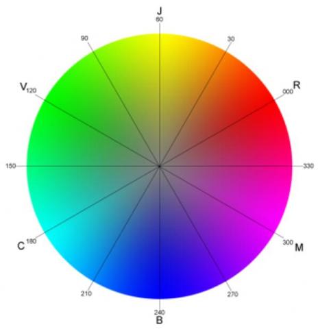
The HSV system (Hue, Saturation, Value) is an image coloring mode that is often more efficient than the classic RGB system (Red, Green, Blue), especially for fractal images. It’s a 3D polar match up a system of hue, saturation and value.
Figure 1. Hue color wheel with degree
-Hue: signifies the illustration of color type. It's expressed by a number which is an angular position on the chromatic wheel 0 to 360 degrees (Figure 1).
Image patches are represented by a histogram over hue computed from the corresponding RGB values of each pixel according to Van de Sande et al. [19] by:
$hue=\arctan \left( \frac{\sqrt{3}\left( R-G \right)}{R+G-2B} \right)$ (19)
To counter instabilities in hue, its impact on the histogram is weighted by the saturation of the corresponding pixel. The hue descriptor is invariant with respect to lighting geometry and specularities when assuming white illumination.
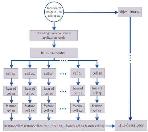
For building our proposed hue descriptor we start first by measuring colors of objects independent the light source color, to make this independence we use the Gray-Edge color constancy, after that we move the image division, in this step we divide our image to 25 cells (sub-image) overlapped by 50%. For each cell we calculate the hue value of each pixel, and by using bin ideas, each cell will be coded with a vector of 12 values. This work will be repeated for all 25 cells. The Final step is regrouping the vectors of cells in one only victor, this vector will be the final characterization victor of the object image (Figure 2).
Figure 2. Building steps of the Hue descriptor
3.1 Step01: Gray-edge color constancy
Color constancy is the ability to recognize colors of objects independent of the color of the light source [33]. Obtaining color constancy is of importance for many computer vision applications, such as image retrieval, image classification, color object recognition and object tracking
Van de Weijer et al. [34], propose a new hypothesis for color constancy namely the Grey-Edge hypothesis, which assumes that the average edge difference in a scene is achromatic. Based on this hypothesis, they propose an algorithm for color constancy. Contrary to existing color constancy algorithms, which are computed from the zero-order structure of images, this method is based on the derivative structure of images. Furthermore, authors propose a framework which unifies a variety of known (Grey-World, max-RGB, Minkowski norm) and the newly proposed Grey-Edge and higher-order Grey-Edge color constancy algorithms. For more details about Gray-Edge color constancy readers will be able to refer to reference [34].
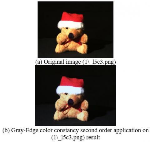
In our descriptor the first step is it’s about applying this Gray-Edge color constancy to make the colors of the object image invariant to light color changes. An example application of this Grey-Edge color constancy is shown in Figure 3.
Figure 3. Gray-edge color constancy second order effects
3.2 Step02: Image division
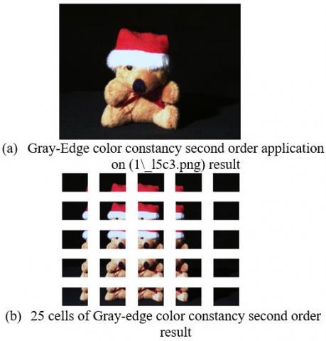
One of the key advantages of the HOG descriptor is its invariance to the geometric and photometric transformation since it operates on local calls [22], in order to keep this invariance to the geometric and photo-metric transformation in our proposed descriptor we used this cell method to make the hue descriptor operate on local calls also. For this reason, and after several studies, we have chosen to divide the object image into 25 cell overlapped by overlapped by 50 % as shown in Figure 4.
Figure 4. Image division result (descriptor cells)
3.3 Step03: Building cell features
In this part, we start first by dividing the hue wheel into 12 parts called bins.
$Huewheel=\left\{ \begin{align} & bin1\cup bin2\cup bin3\cup bin4\cup bin5\cup bin6\cup \\ & bin7\cup bin8\cup bin9\cup bin10\cup bin11\cup bin12 \\ \end{align} \right\}$
with:
$\begin{align} & bin1=\left[ {{0}^{o}},{{29}^{o}} \right],bin2=\left[ {{30}^{o}},{{59}^{o}} \right],bin3=\left[ {{60}^{o}},{{89}^{o}} \right], \\ & bin4=\left[ {{90}^{o}},{{119}^{o}} \right],bin5=\left[ {{120}^{o}},{{149}^{o}} \right],bin6=\left[ {{150}^{o}},{{179}^{o}} \right], \\ & bin7=\left[ {{180}^{o}},{{209}^{o}} \right],bin8=\left[ {{210}^{o}},{{239}^{o}} \right],bin9=\left[ {{240}^{o}},{{269}^{o}} \right], \\ & bin10=\left[ {{270}^{o}},{{299}^{o}} \right],bin11=\left[ {{300}^{o}},{{329}^{o}} \right],bin12=\left[ {{330}^{o}},{{359}^{o}} \right] \\ \end{align}$
After creating the 12 bins, we compute the hue value of each pixel of this cell according to Eq. (19). Then, the vote in bins will be done according to the hues value of each pixel, the magnitude of each bin is calculated by adding the hue magnitudes of all corresponding pixels. In this way we build a feature vector of 12 values (each value from these 12 values corresponds to the magnitude of a bin).
$\text{feature cell 01=}\left[ \begin{align} & \text{magnitude}bin01,\text{magnitude}bin02, \\ & ...,\text{magnitude}bin11,\text{magnitude}bin12 \\ \end{align} \right]$ (20)
3.4 Step04: Histograms normalization
In this paper we used the L2 normalization [20]. Let v be the non-normalized vector containing all histograms in a given block, $\|v\|_{k}$ be its k-norm for k=1,2,... and e be some small constant (the exact value, hopefully, is unimportant). Then the normalization L2 of the vector can be expressed as following:
$f=\frac{v}{\sqrt{\left\| v \right\|_{2}^{2}+{{e}^{2}}}}$ (21)
To get the final feature of cell 01, we normalize the vector cited in Eq. (19) with this L2 normalization.
3.5 Step05: Histograms normalization
To get the final Hue descriptor, steps 3 and 4 are repeated for all cells (25 cells). And then, all cells features will be regrouped in one vector (Figure 2) called ‘Hue descriptor’.
$Hue\text{ }descriptor=\left[ \begin{align} & feature\text{ }cell\text{ }01,\text{ }feature\text{ }cell\text{ }02,\text{ } \\ & \ldots ,\text{ }feature\text{ }cell\text{ }11,\text{ }feature\text{ }cell12 \\ \end{align} \right]$ (22)
All the Hue descriptors (Eq. (22)) of the database images are used to form a classifier of type SVM which generates a model (a set of vectors support). During the phase of the test, the descriptors are calculated in a way identical to the phase of training. Making a decision to join a pattern to its class is performed directly through the decision-making function of the SVM.
4.1 Support vector machine (SVM)
Vladimir Vapnik [35] proposed machine training with vectors of support (Support Vector Machine). From this time, the SVM has been largely used in the pattern recognition; the regression and the estimate of density. We will recall here the elementary principles of this machine.
Suppose a couple $\left(x_{k}, y_{k}\right)$ of random variables of values in $R^{n} \times\{-1,1\}$, where $x_k$ are the Hue descriptors for the examples of training and $y_k$ are the labels of classes. The SVM requires the resolution of the problem of optimization according to:
${{\min }_{w,b,\xi }}\frac{1}{2}{{w}^{T}}w+C\sum\limits_{k=1}^{n}{{{\xi }_{k}}}$ (23)
Under the constraint:
$\begin{matrix} {{y}_{k}}\le \left( {{w}^{T}}+b \right)\ge 1-{{\xi }_{k}} \\ {{\xi }_{k}}\ge 0 \\\end{matrix}$ (24)
where, w is the vector orthogonal to the hyperplane, b is the displacement relative to the origin, $\xi_{k}$ constraint release variables and C it’s balancing variable.
The method consists of transforming the data $x_k$ in a space of dimensions rose due to function φ. The SVM look for a function of optimal decision of the form:
$f\left( x \right)=w.\varphi \left( x \right)+b$ (25)
The kernel function is:
$\left( {{x}_{i}},{{x}_{j}} \right)=\varphi {{\left( {{x}_{i}} \right)}^{T}}.\varphi \left( {{x}_{j}} \right)$ (26)
The basic kernel functions are:
-Linear: the linear kernel function is:
$k\left( {{x}_{i}},{{x}_{j}} \right)={{x}_{i}}^{T}{{x}_{j}}$ (27)
-Polynomial: the polynomial kernel function is:
$k\left( {{x}_{i}},{{x}_{j}} \right)={{\left( \gamma .{{x}_{i}}^{T}{{x}_{j}}+r \right)}^{d}}$ (28)
-Gaussian or RBF (Radial Basis functions): the gaussian kernel function is:
$k\left( {{x}_{i}},{{x}_{j}} \right)=\exp \left( -\gamma {{\left| {{x}_{i}}-{{x}_{j}} \right|}^{2}} \right)$ (29)
-Sigmoid: the sigmoid kernel function is:
$k\left( {{x}_{i}},{{x}_{j}} \right)=\tan \left( \gamma {{x}_{i}}^{T}{{x}_{j}}+r \right)$ (30)
4.2 SVM multi-class
SVM is inherently two class classifier. However, problems in real are in most case multi-class problems, the simplest example is the recognition of the optical characters. In such cases, we do not try to assign a new example to one of the two classes but to one of many classes, i.e. that the decision is no longer binary and a single hyper-plane is not enough anymore.
SVM multi-class separator reduces the multi-class problem to a composition of many two class hyper planes [36, 37]. These methods break down the whole of examples into many subsets; each subset represents a problem of two-class classification. For each problem a hyper-plane of separation is determined by SVM binary method. We build during the classification a hierarchy of the binary hyper-planes which is traversed from root to leaf to decide the class of a new example. There are several methods of decomposition in the literature like SVM one against one proposed by Vapnik [38] and SVM One against all proposed by Knerr et al. [39].
In this paper, we will use SVM multi-class one-against-all with a Gaussian kernel function to classify the descriptors data of the learning base in experiments
In order to evaluate our descriptor, we used two databases, Columbia object image libraries (coil-100) and The Amsterdam Library of Object Images. The first database one will be used for testing the invariance to geometric and photometric transformation, and the second one for studying the invariance to illumination condition changes.
For a detailed comparison between the proposed methodology with some other color-based feature extraction studies, we compare the proposed Hue descriptor results with the results of HOG descriptors, opponent histograms, hue histograms, sift feature and local image descriptors from even Gabor filter responses.
The local image descriptor from even Gabor filter response results are used only in Amsterdam Library of Object Images tests because the source code provides by authors doesn’t support the image size of coil-100($128*128$pixels).
5.1 Image database
In this part we will give a brief presentation about Columbia object image libraries (coil-100) and The Amsterdam Library of Object Images.
5.1.1 Columbia object image library (coil-100)
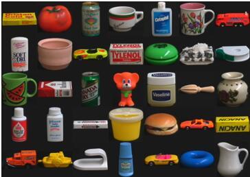
Columbia Object Image library (coil-100) [40] is a database of color images contains 7200 image of 100 objects, 72 different views for each object Images of the objects were taken at pose intervals of 5 degrees, these different angles for each object makes this data set ideal to test the robustness of geometric and photometric transformation. This is why this data set is widely used in object recognition experiments.
Figure 5. Samples of images from the coil-100 database
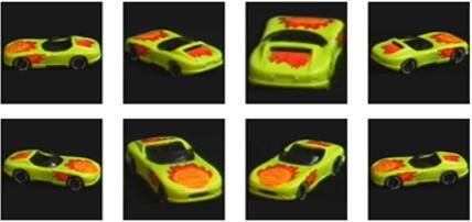
Figure 5 shows some object from the database, while Figure 6 shows the same object with different views.
Figure 6. An object from the coil-100 database with different orientations and scale changes
5.1.2 The Amsterdam Library of object images
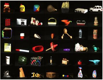
Geusebroek et al. [41], present the ALOI (Amsterdam Library of Object Images) collection of 1,000 objects (Figure 7) recorded under various imaging circumstances. In order to capture the sensory variation in objects recordings, they systematically varied viewing angles, illumination angle (Figure 8), and illumination color for each object (Figure 9), and additionally captured wide-baseline stereo images. They recorded over a hundred images of each object, yielding a total of 110,250 images for the collection. These images are made publicly available for scientific research purposes. The light color is varied by changing the illumination color temperature, resulting in objects illuminated under reddish to white light. For completeness, ALOI dataset are also included objects lighted by a different number of white lights at increasingly oblique angles (between one and three white lights around the object, introducing self shadowing for up to half of the object).
Figure 7. Samples of images from Amsterdam Library of object images
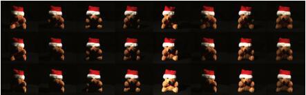
Figure 8. Example object from ALOI viewed under 24 different illumination directions
Figure 9. Example object from ALOI-COL viewed under 12 different illumination color temperatures
5.2 Results
Test step contains 2 parts: the first is Columbia object image library (coil-100) test in which we focus on testing invariance to photometric and geometric transformation, while the Amsterdam Library of Object Images test is dedicated to testing the invariance to the illumination conditions change.
5.2.1 Columbia object image library (coil-100) tests
This experiment is conducted on 34 objects. These 34 objects are chosen by sampling one of each 3 successive objects (we take object number 1 and we don’t take objects number 2 and number 3, we take object number 4 and we don’t take objects number 5 and number 6, …). Through this method, the list of taken object in this experiment from the coil data is (object number1, object number4, object number7, object number 10, object number 13, object number 16, object number 19, object number 22, object number 25, object number 28, object number 31, object number 34, object number 37, object number 40, object number 43, object number 46, object number 49, object number 52, object number 55, object number 58, object number 61, object number 64, object number 67, object number 70, object number 73, object number 76, object number 79, object number 82, object number 85, object number 88, object number 91, object number 94, object number 97 and object number 100).
Since each object has 72 images of different poses (5 degrees apart), we used 22 images for training and 50 for tests for each object from the object list cited before. These 22 images of training are chosen by taking \$15\$ degrees apart.
Each image will be coded using HOG descriptors (HOG), opponent histograms (OPP), hue histograms (Hue H), SIFT features (SIFT), and the Hue descriptor proposed in this paper (Hue dis).
The descriptor parameters used in this experiment are: For HOG histogram 9 is taken as the number of bins and 3 the number of HOG windows per bound box. For Opponent histograms and hue histograms we have used 36 as the number of bins, 2 as smooth flags and lambda=1. For the SIFT feature sigma= $\sqrt{2}$, octave=3 and level=3. While, for the proposed hue descriptor the number of cells is 25 and the number of bins is 12.
To facilitate the result reading, object list is divided into groups, group 01 contains the objects with the number from 1 to 25 (1, 4, 7, 10, 13, 16, 19, 22 and 25). Group 02 contains objects with the number from 28 to 52 (28, 31, 34, 37, 40, 43, 46, 49 and 52). Group 03 contains objects with the number from 55 to 79 (55, 58, 61, 64, 67, 70, 73, 76 and 79) and group contains 04 objects with the number from 82 to 100 (82, 85, 88, 91, 94, 97 and 100).
The classifiers are trained to use all but one image. This last image is used as a test image. In this way, the test image is not used in the training set. Table 1, Table 2, Table 3 and Table 4 give the number of recognized images for each object from a total of 50 images per object used in tests. While, Table 5 represents the average number of recognized images and the recognition rate of experiments carried on Columbia object image library (coil-100) data test. The F1 score value [42] is used to determine the average number of recognized images (ANRI).
$ANRI=\frac{\text{Recognized images}}{\text{Recognized images + Unrecognized images}}$ (31)
Table 1. Number of recognized images for group 01 from a total of 50 images for each object
|
|
HOG [20] |
OPP [19] |
Hue H [19] |
SIFT [30] |
Hue Dis [this article] |
|
Obj01 |
40 |
44 |
45 |
37 |
48 |
|
Obj04 |
41 |
44 |
46 |
40 |
50 |
|
Obj07 |
50 |
48 |
50 |
50 |
50 |
|
Obj10 |
40 |
41 |
42 |
39 |
45 |
|
Obj13 |
39 |
40 |
42 |
38 |
47 |
|
Obj16 |
39 |
43 |
42 |
36 |
48 |
|
Obj19 |
40 |
43 |
45 |
40 |
49 |
|
Obj22 |
40 |
42 |
42 |
39 |
46 |
|
Obj25 |
50 |
50 |
50 |
50 |
50 |
Table 2. Number of recognized images for group 02 from a total of 50 images for each object
|
|
HOG [20] |
OPP [19] |
Hue H [19] |
SIFT [30] |
Hue Dis [this article] |
|
Obj28 |
39 |
40 |
41 |
40 |
44 |
|
Obj31 |
38 |
41 |
42 |
39 |
47 |
|
Obj34 |
50 |
50 |
50 |
50 |
50 |
|
Obj37 |
41 |
40 |
43 |
41 |
47 |
|
Obj40 |
40 |
43 |
44 |
40 |
48 |
|
Obj43 |
38 |
40 |
42 |
39 |
47 |
|
Obj46 |
37 |
40 |
43 |
39 |
46 |
|
Obj49 |
50 |
46 |
50 |
48 |
50 |
|
Obj52 |
38 |
42 |
42 |
39 |
46 |
Table 3. Number of recognized images for group 03 from a total of 50 images for each object
|
|
HOG [20] |
OPP [19] |
Hue H [19] |
SIFT [30] |
Hue Dis [this article] |
|
Obj55 |
38 |
41 |
42 |
39 |
46 |
|
Obj58 |
50 |
45 |
48 |
46 |
50 |
|
Obj61 |
44 |
42 |
45 |
42 |
48 |
|
Obj64 |
39 |
42 |
43 |
40 |
46 |
|
Obj67 |
39 |
42 |
44 |
37 |
48 |
|
Obj70 |
50 |
48 |
48 |
47 |
50 |
|
Obj73 |
50 |
50 |
50 |
48 |
50 |
|
Obj76 |
40 |
42 |
42 |
39 |
47 |
|
Obj79 |
40 |
41 |
42 |
40 |
48 |
Table 4. Number of recognized images for group 04 from a total of 50 images for each object
|
|
HOG [20] |
OPP [19] |
Hue H [19] |
SIFT [30] |
Hue Dis [this article] |
|
Obj82 |
40 |
44 |
48 |
42 |
50 |
|
Obj85 |
39 |
40 |
42 |
38 |
46 |
|
Obj88 |
46 |
44 |
46 |
42 |
50 |
|
Obj91 |
40 |
41 |
42 |
39 |
46 |
|
Obj94 |
50 |
50 |
50 |
50 |
50 |
|
Obj97 |
36 |
41 |
42 |
39 |
46 |
|
Obj100 |
40 |
42 |
44 |
39 |
47 |
From the results shown in Table 5, the proposed Hue descriptor has the best recognition rate in this experiment (95.64%), followed by Hue Histogram (89.36%). The opponent histogram coming third with 86.59% followed by the HOG (84.18%) and the SIFT is last (83.00%).
From the HOG feature and the proposed Hue descriptor results (Table 5), it can be noticed that changing the method of choosing the cell, the number bins and also replacing the arc-tangent used in HOG by the hue values in the proposed Hue descriptor, and also using Gray-Edge color constancy second order applications all this has improved the recognition rate by around 12%. The proposed hue descriptor also has around 13% batter recognition rate then the SIFT feature. This better performance in the proposed is due to the use of color and also due to its strategy of building.
Table 5. Average number of recognized image and the recognition rate of experiments carried on Columbia object image library (coil-100) data test
|
|
Average number of recognized images |
Recognition rate |
|
HOG [20] |
42.09/50 |
84.18% |
|
OPP [19] |
43.29/50 |
86.59% |
|
Hue H [19] |
44.68/50 |
89.36% |
|
SIFT [30] |
41.50/50 |
83.00% |
|
Hue Dis [this article] |
47.82/50 |
95.64% |
From the opponent histogram and the proposed Hue descriptor results, it can be noticed that changing the method of building the feature by using bins and cell ideas, and also by using hue components Gray-Edge color constancy second order applications have made the descriptor more robust against geometric and photometric transformation, this robustness has improved the recognition rate by around 9%.
From the Hue histogram and the proposed Hue descriptor results shown in Table 5, it can be noticed that the proposed Hue descriptor is more efficient than the hue histogram. This efficiency is due to the strategy of building the proposed feature by using cell and bin ideas and also due to using Gray-Edge color constancy second order applications in the proposed feature. This efficiency is clearly shown in the recognition rate of the proposed Hue descriptor which have 6% more than the hue histogram recognition rate.
From the results of Table 5 also, it's observed that for object category recognition, descriptors using color (opponent histogram, hue histograms and the proposed hue descriptor) are more efficient than other methods (HOG and SIFT features).
Table 5 also confirms that the HOG feature is more robust than the SIFT feature against geometric and photometric transformation, this superiority of robustness is because the HOG feature is a local feature since it operates on local calls.
The theoretical properties of hues invariant are confirmed. Features using this component of chrominance (hue histogram and the proposed hue descriptor) have the highest recognition rate.
5.2.2 The Amsterdam Library of object images tests
This experiment is conducted on 26 objects. These 26 objects are chosen by sampling one of each 40 successive objects. Through this method, the list of taken object in this experiment from Amsterdam Library of Object Images data is (object number 1, object number 40, object number 80, object number 120, object number 160, object number 200, object number 240, object number 280, object number 320, object number 360, object number 400, object number 440, object number 480, object number 520, object number 560, object number 600, object number 640, object number 680, object number 720, object number 760, object number 800, object number 840, object number 880, object number 920, object number 960 and object number 1000).
Geusebroek et al. [41], present the Amsterdam Library of Object Images collection of one thousand objects, which we recorded under 72 in plane viewing angles, 24 different illumination angles (Figure 8), and under 12 illumination colors (Figure 9). In this part of experiment, we focus on invariance ton illumination conditions changes. For this for each object we took the images of different illumination angles and different illumination colors, therefore each object has 36 different images. We used 25 images for training, and 7 for tests for each object from the object list cited before. These 7 images of training are chosen by sampling one of each 3 successive images.
Each image will be coded using HOG descriptors (HOG), opponent histograms (OPP), hue histograms (Hue H), SIFT features (SIFT), local image descriptors from even Gabor filter responses (Gabor), and the Hue descriptor proposed in this paper (Hue dis). Parameters of descriptors are the same used in the previous experiments.
Same to the previous experiments, object list is divided into groups, group 01 contains the objects with the number from 1 to 320 (1, 40, 80, 120, 160, 200, 240, 280 and 320). Group 02 contains objects with the number from 360 to 680 (360, 400, 440, 480, 520, 560, 600, 640 and 680) and group 03 contains objects with the number from 720 to 1000 (720, 760, 800, 840, 880, 920, 960 and 1000).
The classifiers are trained to use all but one image. This last image is used as a test image. In this way, the test image is not used in the training set. Table 6, Table 7 and Table 8 represents the number of recognized images for each object from the total of 25 images per object used in tests. While, Table 9 represents the average number of recognized images and the recognition rate of experiments carried on The Amsterdam Library of Object Images data test.
Table 6. Number of recognized images for group 01 from a total of 25 images for each object
|
|
HOG [20] |
OPP [19] |
Hue H [19] |
SIFT [30] |
GABOR [32] |
Hue Dis [this article] |
|
Obj01 |
20 |
21 |
22 |
20 |
22 |
23 |
|
Obj40 |
23 |
23 |
23 |
22 |
23 |
24 |
|
Obj80 |
21 |
21 |
22 |
20 |
23 |
23 |
|
Obj120 |
23 |
22 |
23 |
22 |
24 |
25 |
|
Obj160 |
21 |
22 |
22 |
20 |
22 |
24 |
|
Obj200 |
21 |
21 |
22 |
20 |
21 |
23 |
|
Obj240 |
19 |
20 |
20 |
19 |
21 |
22 |
|
Obj280 |
20 |
20 |
21 |
20 |
22 |
24 |
|
Obj320 |
22 |
22 |
23 |
21 |
23 |
24 |
Table 7. Number of recognized images for group 02 from a total of 25 images for each object
|
|
HOG [20] |
OPP [19] |
Hue H [19] |
SIFT [30] |
GABOR [32] |
Hue Dis [this article] |
|
Obj360 |
22 |
23 |
24 |
22 |
24 |
24 |
|
Obj400 |
21 |
21 |
22 |
20 |
22 |
23 |
|
Obj440 |
21 |
22 |
23 |
20 |
23 |
23 |
|
Obj480 |
22 |
23 |
24 |
22 |
24 |
24 |
|
Obj520 |
20 |
21 |
21 |
19 |
22 |
23 |
|
Obj560 |
19 |
21 |
21 |
20 |
21 |
23 |
|
Obj600 |
20 |
20 |
21 |
19 |
21 |
22 |
|
Obj640 |
20 |
21 |
21 |
20 |
22 |
23 |
|
Obj680 |
21 |
22 |
22 |
21 |
22 |
23 |
|
|
HOG [20] |
OPP [19] |
Hue H [19] |
SIFT [30] |
GABOR [32] |
Hue Dis [this article] |
|
Obj720 |
21 |
22 |
23 |
21 |
23 |
24 |
|
Obj760 |
20 |
20 |
22 |
19 |
22 |
23 |
|
Obj800 |
20 |
21 |
22 |
19 |
21 |
23 |
|
Obj840 |
21 |
21 |
22 |
21 |
23 |
23 |
|
Obj880 |
19 |
20 |
20 |
18 |
20 |
21 |
|
Obj920 |
20 |
20 |
22 |
20 |
22 |
23 |
|
Obj960 |
20 |
21 |
22 |
20 |
21 |
23 |
|
Obj1000 |
19 |
21 |
22 |
19 |
23 |
23 |
Table 9. Average number of recognized image and the recognition rate of experiments carried on the Amsterdam Library of object images
|
|
Average number of recognized images |
Recognition rate |
|
HOG [20] |
20.62/25 |
82.46% |
|
OPP [19] |
22.08/25 |
88.32% |
|
Hue H [19] |
22.88/25 |
91.52% |
|
SIFT [30] |
20.96/25 |
83.84% |
|
GABOR [32] |
23.08/25 |
92.32% |
|
Hue Dis [this article] |
24.12/25 |
96.48% |
From the results shown in Table 9, the proposed Hue descriptor has the best recognition rate in this experiment (96.48%), followed by GABOR features (92.32%). Hue Histogram coming third with 91.52% followed by the opponent histogram (88.32%) and the SIFT feature (83.84%). HOG recognition rate is the last with 82.46%.
HOG feature is sensitive to illumination condition change, like change in the illumination color and light scattering, shadows and lighting geometry changes such as shading and the highlights under a white light source and scattering of a white source, all this, can operate significantly the recognition rate of this method. The proposed Hue descriptor solve this lack of invaiance by Hue which is invariant to shadows and lighting geometry changes such as shading and the highlights under a white light source and scattering of a white source, and also by using Gray-Edge color constancy second order which solve the problem of missing invariance to change in the illumination color and light scattering. This invariance added have improved the recognition rate with around 14% (Table 5).
The SIFT feature is not invariant to light color changes (change in the illumination color and light scattering), the proposed Hue descriptor solve this problem by using Gray-Edge color constancy second order. This invariance added can be clearly noticed from the difference in the recognition rate shown in table5 (the proposed hue descriptor rete is highest by around 12%).
The proposed hue descriptor solves the drawbacks of opponent histograms by using the hue which is invariant to light intensity change (change in shadows and lighting geometry changes such as shading), light intensity shift (objects highlights under a white light source and scattering of a white source) and light intensity change and shift (combinations of the above two conditions), and also the Gray-Edge color constancy to solve the problem of missing invariance to the light color change (change in the illumination color and light scattering). This invariance added have improved the recognition rate of the opponent histogram with around 12% as shown in Table 5.
As it mentioned before, the hue histogram is invariant to changes in the illumination color and light scattering. The proposed hue descriptor solves this miss of invariance by using Gray-Edge color constancy second order. Thing that has improved the recognition rate with around 5%.
Even if Zambanini and Kampel [32], present their descriptors as a local descriptor robust to illumination Changes, but this experiment results show that combination of Gray-Edge color constancy, hue components and cell and bin ideas give a descriptor more efficient.
From the results of Table 9, the theoretical invariance properties of color descriptors are validated. By observing the results with respect to illumination conditions changes, the color descriptors without invariance to this property, such as the opponent histogram do not perform well. There is a clear distinction in performance between these descriptors and the invariant descriptors, such as the hue histogram and the proposed hue descriptor. Overall, descriptors using color perform much better than the HOG and SIFT descriptors.
In this paper, a new color object recognition model has been proposed which is analyzed in theory and evaluated in practice for the purpose of recognition of multicolored objects invariant to a substantial change in illumination and also photometric and geometric transformation. The proposed oriented descriptor benefits of the invariance of hues against light intensity change, light intensity shift and light intensity change and shift, and solve its missing of invariance against light color change by using Gray-Edge color constancy. Moreover, the use of cells and bins in this proposed descriptor building boost its invariance the geometric and photo-metric transformation and increases the recognition rate. This idea is based on measuring colors of objects independent of the light source color by using color constancy, and then dividing the image into twenty-five cells overlapped by 50% to make the descriptor operate on local calls. Cells feature is building by calculates the hue value on each pixel and allocating the magnitude of hues in twelve bins, by grouping this bins-magnitude values in a vector, we get a characterization feature for the cell, then, after feature normalization, and by grouping all the twenty-five cells features in one vector we get the final descriptor of images. SVM classifiers (Support Vector Machine) which is a strong classification method known for its flexibility and its power of generalization are used for the training and recognition steps. The proposed method is evaluated on two publicly available datasets including Columbia Object Image Library and The Amsterdam Library of Object Images and obtained a recognition rate of 95.64% and 96.64% - clearly showing the exceptional performance compared to existing methods. This also shows that this model of recognition is promising and could be the subject of industrial applications. Changing the type of data (for example using the proposed feature to detect pedestrians (human) or some other objects such as car, dog, cat, etc., or using non-uniform background) will be the subject of our future works. We are also aiming that the feature proposed in this paper will be the base of an application that will replace the use of bar code in commercials store (mall, pharmacies …, etc.).
[1] Feng, Q., Hao, Q., Sbert, M., Yi, Y., Wei, Y., Dai, J. (2019). Local parallel cross pattern: A color texture descriptor for image retrieval. Sensors, 19(2): 315. http://dx.doi.org/10.3390/s19020315
[2] Ahmed, K.T., Naqvi, S.A.H., Rehman, A., Saba, T. (2019). Convolution, approximation and spatial information based object and color signatures for content based image retrieval. In 2019 International Conference on Computer and Information Sciences (ICCIS), Sakaka, Saudi Arabia, pp. 1-6. http://dx.doi.org/10.1109/ICCISci.2019.8716437
[3] Dad, N., En-nahnahi, N., Ouatik, S.E.A. (2019). Quaternion Harmonic moments and extreme learning machine for color object recognition. Multimedia Tools and Applications, 78(15): 20935-20959. http://dx.doi.org/10.1007/s11042-019-7381-2
[4] Wei, X.S., Zhang, C.L., Wu, J., Shen, C., Zhou, Z.H. (2019). Unsupervised object discovery and co-localization by deep descriptor transformation. Pattern Recognition, 88: 113-126. http://dx.doi.org/10.1016/j.patcog.2018.10.022
[5] Susan, S., Agrawal, P., Mittal, M., Bansal, S. (2019). New shape descriptor in the context of edge continuity. CAAI Transactions on Intelligence Technology, 4(2): 101-109. http://dx.doi.org/10.1049/trit.2019.0002
[6] Lin, G., Tang, Y., Zou, X., Xiong, J., Fang, Y. (2019). Color-, depth-, and shape-based 3D fruit detection. Precision Agriculture, 1-17. http://dx.doi.org/10.1007/s11119-019-09654-w
[7] Swain, M., Ballard, D. (1991). Color indexing. International Journal of Computer Vision, 7(1): 11-32. https://doi.org/10.1007/BF00130487
[8] Funt, B., Finlayson, G. (1995). Color constant color indexing. IEEE Transactions on Pattern Analysis and Machine Intelligence, 17(5): 522-529. http://dx.doi.org/10.1109/34.391390
[9] Land, E., McCann, J. (1971). Lightness and retinex theory. Journal of the Optical Society of America, 61(1): 1-11. http://dx.doi.org/10.1364/JOSA.61.000001
[10] Healey, G., Slater, D. (1995). Global color constancy: Recognition of objects by use of illumination invariant properties of color distribution. Journal of the Optical Society of America, 11(11): 3003-3010. http://dx.doi.org/10.1364/JOSAA.11.003003
[11] Finlayson, D., Chatterjee, S., Funt, B. (1996). Color angular indexing. ECCV’1996 European Conference on Computer Vision, Berlin, Heidelberg, pp. 16-27. http://dx.doi.org/10.1007/3-540-61123-1_124
[12] Slater, D., Healey, G. (1996). The illumination-invariant recognition of 3-D objects using local color invariants. IEEE Transactions on Pattern Analysis and Machine Intelligence, 18(2): 206-211. http://dx.doi.org/10.1109/34.481544
[13] Hoiem, D., Chodpathumwan, Y., Dai, Q. (2012). Diagnosing error in object detectors. ECCV, pp. 340-353. https://doi.org/10.1007/978-3-642-33712-3_25
[14] Felzenszwalb, P., Girshick, R., Mcallester, D., Ramanan, D. (2010). Object detection with discriminatively trained part-based models. IEEE Transactions on Pattern Analysis and Machine Intelligence, 32(9): 1627-1645. http://dx.doi.org/10.1109/TPAMI.2009.167
[15] Uijlings, J.R.R., van de Sande, K.E.A., Gevers, T., Smeulders, A.W.M. (2013). Selective search for object recognition. International Journal of Computer Vision, 104(2): 154-171. http://dx.doi.org/10.1007/s11263-013-0620-5
[16] Girshick, R., Donahue, J., Darrell, T., Malik, J. (2013). Rich feature hierarchies for accurate object detection and semantic segmentation. Proceedings of the IEEE Computer Society Conference on Computer Vision and Pattern Recognition. http://dx.doi.org/10.1109/CVPR.2014.81
[17] Gevers, T., Smeulders, A. (1998). Color-based object recognition. Pattern Recognition Journal, 32(3): 453-464. http://dx.doi.org/10.1016/S0031-3203(98)00036-3
[18] Von Kries, J. (1970). In Influence of Adaptation on the Effects Produced by Luminous Stimuli. Sources of Color Vision: MIT Press, Cambridge.
[19] Van de Sande, K., Gevers, T., Snoek, C. (2010). Evaluating color descriptors for object and scene recognition. IEEE Transactions on Pattern Analysis and Machine Intelligence, 32(9): 1582-1596. http://dx.doi.org/10.1109/TPAMI.2009.154
[20] Dalal, N., Triggs, B. (2005). Histograms of oriented gradients for human detection. In IEEE 2005 CVPR’05 Computer Society Conference on Computer Vision and Pattern Recognition, San Diego, CA, USA, pp. 886-893. http://dx.doi.org/10.1109/CVPR.2005.177
[21] Dalal, N. (2006). Finding people in images and videos. Ph.D. The National Polytechnic Institute of Grenoble, France.
[22] Ilas, M., Ilas, C. (2018). A new method of histogram computation for efficient implementation of the HOG algorithm. Computers, 7: 3-18. http://dx.doi.org/10.3390/computers7010018
[23] Lee, S.H., Bang, M., Jung, K., Yi, K. (2015). An efficient selection of HOG features for SVM classification of vehicle. in IEEE 2015 ISCE International Symposium on Consumer Electronics, Madrid, Spain, pp. 24-26. http://dx.doi.org/10.1109/ISCE.2015.7177766
[24] Li, X., Guo, X. (2013). A HOG feature and SVM based method for forward vehicle detection with single camera. In IHMSC 5th International Conference on Intelligent Human-Machine Systems and Cybernetics, Hangzhou, China, pp. 263-266. http://dx.doi.org/10.1109/IHMSC.2013.69
[25] Hsiao, P., Lin, S., Huang, S. (2015). An FPGA based human detection system with embedded platform. Microelectronic Engineering, 138: 42-46. http://dx.doi.org/10.1016/j.mee.2015.01.018
[26] Bauer, S., Köhler, S., Doll, K., Brunsmann, U. (2010). FPGA-GPU architecture for kernel SVM pedestrian detection. In IEEE 2010 CVPRW Computer Society Conference on Computer Vision and Pattern Recognition Workshops, San Francisco, CA, USA, pp. 61-68. http://dx.doi.org/10.1109/CVPRW.2010.5543772
[27] Bauer, D., Brunsmann, U., Schlotterbeck-Macht, S. (2009). FPGA implementation of a HOG-based pedestrian recognition system. In MPC-Workshop, Karlsruhe, Germany, pp. 49-58.
[28] Van de Weijer, J., Schmid, C. (2006). Coloring local feature extraction. In 9th European Conference on Computer Vision, Graz, Austria, 7-13, Proceedings, Part II, pp. 334-348. http://dx.doi.org/10.1007/11744047_26
[29] Van de Weijer, J., Gevers, T., Bagdanov, A. (2006). Boosting color saliency in image feature detection. IEEE Transactions on Pattern Analysis and Machine Intelligence, 28(1): 150-156. http://dx.doi.org/10.1109/TPAMI.2006.3
[30] Lowe, D.G. (2004). Distinctive image features from scale-invariant key points. International Journal of Computer Vision, 60: 91-110. https://doi.org/10.1023/B:VISI.0000029664.99615.94
[31] Daugman, J.G. (1985). Uncertainty relation for resolution in space, spatial frequency, and orientation optimized by two-dimensional visual cortical filters. Journal of the Optical Society of America A, 2: 1160-1169. http://dx.doi.org/10.1364/JOSAA.2.001160
[32] Zambanini, S., Kampel, M. (2013). A local image descriptor robust to illumination changes. in Kämäräinen J.K, Koskela M. (Eds) Image Analysis. SCIA 2013. Lecture Notes in Computer Science, 7944. Springer, Berlin, Heidelberg. http://dx.doi.org/10.1007/978-3-642-38886-6_2
[33] Forsyth, D. (1990). A novel algorithm for color constancy. International Journal of Computer Vision, 5: 5-36. http://dx.doi.org/10.1007/BF00056770
[34] Van de Weijer, J., Gevers, T., Gijsenij, A. (2007). Edge-based color constancy. IEEE Transactions on Image Processing, 16(9): 2207-2214. http://dx.doi.org/10.1109/TIP.2007.901808
[35] Vapnik, V. (1995). The Nature of Statistical Learning Theory. Springer-Verlag: Berlin, Heidelberg. http://dx.doi.org/10.1007/978-1-4757-2440-0
[36] Hamel, L. (2009). Knowledge discovery with support vector machines. Wiley Edition: New York, NY, USA. http://dx.doi.org/10.1002/9780470503065
[37] Shigeo, A. (2005). Support Vector Machines for Pattern Classification. Springer-Verlag: London. https://doi.org/10.1007/1-84628-219-5
[38] Vapnik, V. (1998). Statistical Learning Theory. Wiley Edition: New York, NY, USA.
[39] Knerr, S., Personnaz, L., Dreyfus, J. (1990). Single-layer learning revisited: a stepwise procedure for building and training a neural network. Soulié F.F., Hérault J. Eds., Springer: Berlin, Heidelberg, 41-50. http://dx.doi.org/10.1007/978-3-642-76153-9_5
[40] Nene, S.A., Nayar, S.K., Murase, H. (1996). Columbia Object Image Library (COIL-100). Technical Report CUCS -006-96, Columbia Univ.
[41] Geusebroek, J.M., Burghouts, G., Smeulders, A. (2005). The Amsterdam library of object images. International Journal of Computer Vision, 61: 103-112. http://dx.doi.org/10.1023/B:VISI.0000042993.50813.60
[42] Goutte, C., Gaussier, E. (2005). A probabilistic interpretation of precision, recall and F-score, with implication for evaluation. In European Conference on Information Retrieval, 345-359. Springer, Berlin, Heidelberg. http://dx.doi.org/10.1007/978-3-540-31865-1_25