OPEN ACCESS
The mirrors of a traditional Fresnel system are moved with a tracking system that allows rotation around a single axis. However, this type of movement in the LFR generates high losses at its ends. The paper aims to study a configuration in which the primary reflectors that generate the aforementioned losses are made movable around two axes to increase the efficiency of the plant.
The work presents the kinematic system for moving the field of mirrors in which the control of solar tracking is carried out with the open loop technique. From a constructive point of view, the mechanical components necessary for the purpose are identified. To allow a robust solar tracking, not influenced by external forces, the rotation of the mirrors is managed by "stepper" type servomotors.
In particular, the use of the aforementioned motors generates a motion by steps, of which it is necessary to know in detail the temporal characteristics and the driving logic of the motors. The behavior of the whole set of "electric motor - mechanical system" will be modeled numerically in order to define the control logic of the servomotor that allows the execution of the steps at the right moment, evaluating the torque and the errors in the motion. In fact, the adoption of too small pitches improves solar tracking but needs the presence of a complex reduction system, with numerous gear wheels, which requires too high torque values.
linear Fresnel reflectors, stepper, biaxial movement
Concentrated solar power plants or CSP (Concentrating Solar Power) convert solar radiation into thermal energy, using reflective surfaces, which focus the sun's rays on a smaller receiver [1]. A concentrator and receiver constitute the solar collector, equipped with a tracking system that allows it to follow the apparent motion of the Sun [2].
Concentration plants are distinguished, based on their intended use, into solar thermal systems and thermodynamic solar systems. The first allow the absorption and eventually accumulation of thermal energy thanks to a heat transfer fluid, to then be used for industrial or domestic purposes. In the latter, a thermodynamic cycle is added to the incident solar energy collection phase (usually a Stirling cycle or a Rankine cycle) for the transformation of the thermal energy collected into electricity, via an alternator [3].
As regards the costs of the electricity produced, only the initial investment costs and maintenance costs affect them, as solar radiation is exploited as the primary source. In the future it is expected, however, that they can be further reduced thanks to the entry on the market of an increasing number of suppliers [4].
Among the most widespread solar concentration plants, which differ from the others also due to the lower initial cost, there are those that use Fresnel linear collectors.
The concentrator consists of segments of flat or slightly curved mirrors arranged according to the principle of the Fresnel lens [5]. The receiver tube is positioned at the focal point and is fixed; unlike the linear parabolic collector, the movement therefore concerns only the concentrator. This is an advantage because, to let the heat transfer fluid circulate, the use of flexible hoses in the connection between the individual manifolds and between these and the pipes of the distribution network is avoided.
To reduce the dispersion of the reflected light, numerous studies have been carried out on the geometries of a secondary reflective surface to be installed above the tube to re-concentrate the rays [6]. The absorber tube is crossed by molten salts or diathermic oil that heat up, or by water that evaporates producing steam, which is sent into a turbine for the direct production of electricity.
The primary reflection system is composed of mirrors arranged parallel on a plane. Mirrors vary in size according to the size of the installation; they can even reach 1.5 m in width and 5 m in length. The efficiency of the system is determined very much by the reflectivity of the mirrors; it must be high, not only during the realization phase, but also during the whole life of the mirror [7]. There are different solutions regarding the creation of the reflecting surface of the primary panels. Today, silver surfaces are often used, protected by glass and multilayer paints, which are applied to the rear of the reflective side to protect it from the effect of external agents that cause aging and loss of performance over time.
Among the losses that limit the optical efficiency of the system, in addition to the optical losses due to the properties of the reflecting surfaces and the absorber glass, there are also others caused by the movement of the reflectors.
These include losses due to blocking, shading, for extremes and for the error in the non-continuous motion that is followed.
Losses due to blocking and shading can be reduced by increasing the distance between adjacent reflectors [8]. However, this solution limits the area actually occupied by the plant. Alternatively, you can keep the distance between the spotlights unchanged and accept that they do not produce useful effects at certain times of day.
End losses, on the other hand, are inevitable with primary reflectors able to rotate around a single axis [9]. In this work, a type of system will be proposed in which the reflectors placed at the longitudinal ends of the plant have two degrees of freedom so as to reduce them as much as possible.
As mentioned, there are also losses due to tracking errors. The motors used in moving the mirrors are steppers. This implies that the law of the following motion must be carried out by means of a step-wise course, which inevitably does not allow perfect directing of the sun's rays towards the tube.
In this work, the stepper motors will be modelled from the electromechanical point of view, in order to identify the characteristics that allow optimization of the energy yield while guaranteeing effective solar tracking.
End losses in a linear Fresnel system are very important as they directly affect the overall optical efficiency. They are determined a lot by the position of the Sun on the celestial vault and, therefore, vary according to the time and the period of the year.
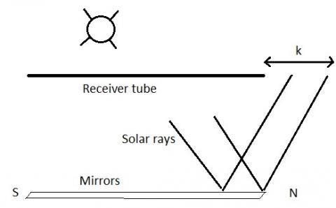
With reference to a plant oriented in a North-South direction, Figure 1 shows that, when the sun on the sky is in a longitudinal direction to the plant (for example at noon), a substantial part of the pipe is not radiated by the sun's rays.
Figure 1. End losses
A solution often adopted consists in constructing the plant in such a way that the pipe has a greater longitudinal length than the dimensions of the reflectors. However, this solution does not improve the collector efficiency. In fact, for the same area available for the plant, the final part of the ground is occupied only by the protrusion of the pipe and is therefore not covered by reflectors. To exploit all the available surface it is advisable that it is completely covered with reflectors. In this way, inevitably, the tube cannot exceed the length of the reflectors, which already cover the entire area of the plant.
In a traditional Fresnel linear system, the end losses are caused by the solar tracking system which allows the reflectors to be rotated only around an axis. The law of motion of reflectors is the following [8]:
β=90∘−arctan√1−cos2αcos2a−sinαcosαsin a+12arctandh (1)
In Eq. (1), β represents the angle between the normal of the reflector and the horizontal direction East; d is the distance of the reflector from the center of the plant; h is the height of the tube from the plane of the mirrors; a and α are the azimuth and the solar altitude respectively.
From the correlation it is evident that all the mirrors rotate at the same angle. The rotation, in fact, is exclusively determined by the solar parameters to which is added a fixed term dependent only on the row of mirrors considered.
During reflection, the point of arrival on the pipe is not on the same cross-section as the point where the reflection takes place. With reference to the final part of the system, it happens that the reflected rays, owing to this phase shift, do not hit the receiver. Once k is defined as the aforementioned length, therefore, it is the portion of the plant in which the reflective surfaces do not provide useful effect. Its value is obtained by studying the reflection deriving from the movement with the law of Eq. (1) [9]:
k=cosαcosa√1−cos2αcos2a⋅√d2+h2 (2)
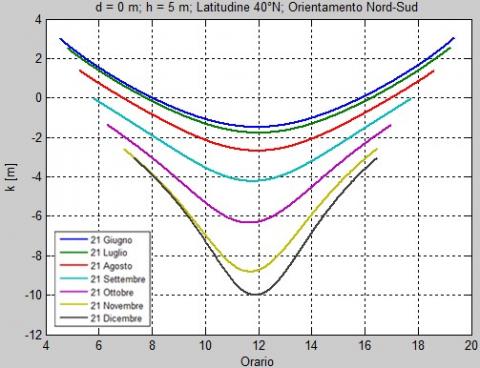
Therefore, according to the height of the pipe, the end losses can reach significant values. Figure 2 shows the trend of the length k obtained by applying Eq. (2) in the case of a plant with a North-South orientation and a receiver tube height of 5 meters.
Figure 2. k length for different days. h = 5 m Orientation North-South
It is noted that, for June 21, k is between -2 meters and 2 meters, while, for December 21, it also reaches values of 10 meters at noon.
To eliminate the losses caused by the end effects, a system with two degrees of freedom is studied, applied only to the reflectors placed in the end parts of the collector.
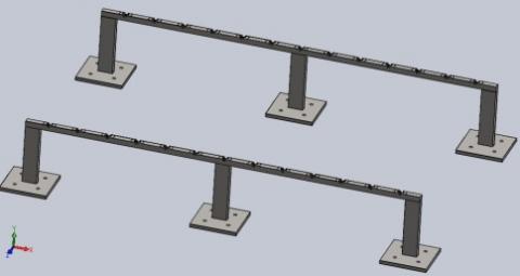
The structure consists of supporting bases on which are placed horizontal steel beams that have the function of supporting the mirrors and the corresponding supports.
The bases have a vertical shape; they are anchored to the ground through a square steel base as shown in Figure 5.a. They are used to support the horizontal steel beams that are arranged in a transverse direction with respect to the plant.
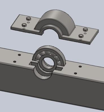
On the beams there are grooves (Figure 3) necessary to insert the bearings that allow the rotation of the mirrors along their main axis.
Figure 3. Detail of the beam with bearing
There are two support tracks to accommodate two bearings. Based on the size of the installation, and in particular on the length k described in the previous paragraph, the section of the installation to be covered with reflectors with two degrees of freedom is determined.
In order to be sure of recovering all the end losses, the section must have a length equal to the maximum value that k assumes over the entire year and, in order to avoid using excessively long reflectors, it is covered with numerous mirrors lower in length. On the beams there is the housing for two bearings: to allow, on both sides, the installation of reflectors that can be moved around two axes. The bearings are then protected by the bearing covers.
The mirrors able to rotate around two axes are mounted between the two horizontal beams. In particular, in the configuration presented, the installation of 13 primary reflectors is planned. A main rotation takes place around the axis passing between the two bearings of the two beams. The secondary rotation, instead, takes place around an axis perpendicular to the main axis; this axis, in turn, rotates undergoing the primary rotation.
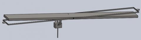
The secondary rotation axis consists of a rod, inserted on the support, which rotates integrally with the latter. The support is shown in Figure 4.a.
The support, therefore, is embedded at its longitudinal ends on the inner rings of the bearings, which guarantee primary movement. The mirror is supported by the transversal central rod and is able to perform the secondary rotation around this axis.
In a decentralized position, as shown in Figure 4.a, the servomotor housing is connected to the support. In fact, the motor that generates the secondary rotation must rotate together with the entire support. The rotary servomotor, by means of a "gear wheel-rack" system, transfers the motion to the mirror pushing it upwards or pulling it downwards. The decentralized position to which the motor is placed allows the reflector to be moved, in the secondary direction, through the application of a suitably calibrated torque, to guarantee the correct positioning of the mirror.
Figure 4.b shows the coupling between the support and the mirror. The mirror is hinged on the central rod. The linear motion is achieved by means of a vertical rod with the function of pushing and/or pulling the reflector.
(a)
(b)
Figure 4. (a) Reflector support, (b) Primary reflector mounted on the support
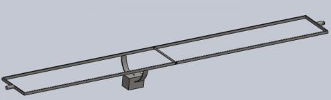
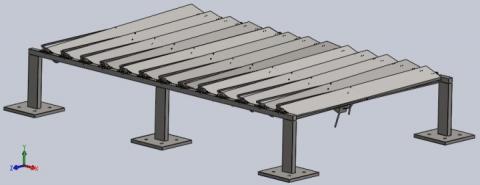
Finally, Figure 5 shows the complete representation of the concentrator positioned at the two ends of the plant.
(a)
(b)
Figure 5. (a) Main elements of the supporting structure, (b) Field of biaxial mirrors
The inclinations that the biaxial mirrors must assume to reflect the radiation exactly on the point of the tube belonging to the same cross-section as the point where the reflection takes place are determined in [9]. They are the following:
θP=arctan(−sinθatanθα) (3)
θq=−arcsin(cosθαcosθa) (4)
In which θ_P represents the angle of the primary rotation, θ_q the angle of the secondary rotation, θ_a the azimuth of the normal to the surface and θ_α the angular altitude of the same with respect to the horizon. The expressions for the calculation of these last two quantities are the following:
{{\theta }_{a}}=\arctan \frac{\frac{h\cdot \left( d\cdot {{z}_{S}}-h\cdot {{x}_{S}} \right)}{\sqrt{{{d}^{2}}+{{h}^{2}}}}-d\cdot \left( y_{S}^{2}+z_{S}^{2} \right)+{{x}_{S}}{{z}_{S}}h}{d\cdot {{x}_{S}}{{y}_{S}}+h\cdot {{y}_{S}}{{z}_{S}}-{{y}_{S}}\sqrt{{{d}^{2}}+{{h}^{2}}}} (5)
{{\theta }_{\alpha }}=\arctan \left( \frac{h}{d}\cdot \sin {{\theta }_{a}}+\frac{d\cdot {{z}_{S}}-h\cdot {{x}_{S}}}{d\cdot {{y}_{S}}}\cdot \cos {{\theta }_{a}} \right) (6)
where, xS, yS and zS are the spatial coordinates of the versor representing the direction of the solar rays.
Unlike classic LFRs, the rotation angles of the different mirrors are not equal in the reflectors moved around two axes, and it is for this reason that two servomotors should be used for each reflector. The use of two servomotors for each reflector would lead to an increase in the initial cost of the plant, making its installation uneconomical.
However, for a system oriented towards the North-South direction, the trends of the θ_P for the various reflectors are very similar to each other during the day. It is therefore possible, by accepting a minimum error, to perform the primary rotations of the reflectors with the same servomotor, adopting the law of motion of the central reflector. Regarding instead the secondary rotation it is necessary to insert a servomotor for each reflector, which rotates together with it solidly.
For the sizing of the servomotors and the possible error deriving from the application of a stepper motor, the need arises to analyze the dynamics of interaction between the electric part constituted by the motor and the mechanical part represented by the reflector, which opposes the rotation motion based on its rotational inertia.
On the basis, therefore, to these premises, the actuator consists of a two-phase bipolar hybrid stepper motor for which a control model has been created.
In short, it is composed of windings in the stator crossed by current so as to generate a magnetic field; the rotor is made up of a permanent magnet that rotates placing its poles in the opposite direction to the generated magnetic field. By alternately feeding the windings it is possible to make the rotor perform small steps. For driving the actuator, in One phase on mode, the current must always be present in both phases, but changing towards. The result is that the torque increases about 1.4 times and the current absorbed doubles. In Table 1 the alternation of the current in the phases is shown to allow the execution of four steps, with reference to a motor with four polar expansions.
Table 1. Current alternation in phases
|
Step |
Phase 1 |
Phase 2 |
|
1 |
1 |
0 |
|
2 |
0 |
-1 |
|
3 |
-1 |
0 |
|
4 |
0 |
1 |
The equations necessary to describe the electrical operation of the hybrid stepper motor are as follows:
{{V}_{a}}={{L}_{a}}\frac{d{{i}_{a}}}{dt}+R\cdot {{i}_{a}}-{{k}_{e}}\cdot \omega \cdot \sin (\theta \cdot {{N}_{c}}) (7)
{{V}_{b}}={{L}_{b}}\frac{d{{i}_{b}}}{dt}+R\cdot {{i}_{b}}-{{k}_{e}}\cdot \omega \cdot \cos (\theta \cdot {{N}_{c}}) (8)
C=-{{k}_{e}}\cdot {{i}_{a}}\cdot \sin (\theta \cdot {{N}_{c}})-{{k}_{e}}\cdot {{i}_{b}}\cdot \cos (\theta \cdot {{N}_{c}}) (9)
in which:
a and b subscripts refer to the two phases;
L_a and L_b are the inductances of the phase windings;
V_a and V_b are the voltages of the two phases;
{{i}_{a}} and {{i}_{b}} are the currents flowing in the two windings;
R is the resistance of the electrical circuit of each phase;
{{k}_{e}} is the torque conversion factor [Nm/A];
ω is the angular velocity of the rotor;
ϴ is the angular position of the rotor;
Nc is the number of polar pairs of the rotor;
C is the generated torque.
The electrical equations to the meshes, Eq. (7) and (8), indicate that the supply voltage is distributed in: inductive voltage drop on the winding, voltage drop caused by the resistance of the electric circuit and induced electromotive force which generates the torque that allows rotor rotation. Eq. (9) derives from the Lorentz law and expresses the torque acting on the rotor, as a function of the position of the rotor itself, and of the intensity of current flowing through the windings. To these equations it is necessary to add others that are representative of the load to be moved.
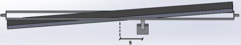
First of all, with reference to the motor that generates secondary rotation, the transmission system must be taken into account, for which, as already mentioned, the coupling of gear wheel and rack is used. By indicating the radius of the toothed wheel with r and the distance between the center of the reflector and the point where the servomotor is positioned with s (Figure 6), it is possible to write the second cardinal equation of the dynamics:
\frac{C}{r}\cdot s={{J}_{p}}\frac{d{{\omega }_{p}}}{dt} (10)
in which:
J_p represents the moment of polar inertia with respect to the axis to which the panel is hinged. It is given by the following relationship:
{{J}_{p}}=\frac{M}{12}\cdot ({{l}^{2}}+s{{p}^{2}}) (11)
where, M represents the mass of the panel, l the length and sp the thickness.
ω_p represents, instead, the angular speed of the panel.
Figure 6. Position of the servomotor
The mechanical link between the rotation angle of the rotor and the angle of inclination of the panel with respect to the horizontal position provides another correlation. The linear vertical movement that the rack undergoes is given by:
\Delta L=r\cdot \Delta \theta (12)
The same displacement, with reference to the panel, can be expressed as:
\Delta L=s\cdot \tan \theta '{{'}_{p}}-s\cdot \tan \theta {{'}_{p}}=s\cdot \Delta \tan {{\theta }_{p}} (13)
where, \theta _{p}^{''} indicates the final angle reached by the panel and \theta _{p}^{'} the initial angle.
By equating Eq. (12) and (13) and deriving, it is obtained:
r\cdot \frac{d\theta }{dt}=s\cdot \frac{d\tan {{\theta }_{p}}}{dt} (14)
Then:
r\cdot \omega =s\cdot \frac{{{\omega }_{p}}}{{{\cos }^{2}}{{\theta }_{p}}} (15)
Eq. (15) represents the link between the angular velocity of the rotor and the angular velocity of the panel. This is not a linear type of link since the position angle of the panel also appears in the correlation. The calculations that are reported below refer to a panel with the geometric characteristics summarized in Table 2.
Table 2. Geometric and mass characteristics of a primary reflector
|
length l |
1.5 m |
|
thickness sp |
0.05 m |
|
density ρ |
800 kg/m3 |
|
mass M |
18 kg |
|
r |
2.5 mm |
|
s |
0.3 m |
|
J_p |
3.37 kg ∙ m2 |
Table 3. Electrical characteristics of the stepper motor
|
Rated voltage ΔV |
3.1 V |
|
Rated current I |
5.5 A |
|
Phase inductances L_a and L_b |
0.0018 H |
|
Phase resistances R_a and R_b |
0,1 Ω |
|
Number of rotor teeth |
50 |
|
Number of polar expansions |
4 |
|
angular step |
1.8° |
|
torque conversion factor ke |
0.5 Nm/A |
The value of r is important because it is determined by the performance of numerous rotations by the panel covering small angles. Of course, in reality, the rotor radius does not have such a low value of r (2.5 millimetres). To reduce the value of r, inside the transmission, it is necessary to insert a speed reducer. The insertion of the reducer allows the torque to be increased and, at the same time, the output speed to be reduced. It is possible to obtain a reduction factor of about 10 (assuming the rotor radius is approximately 2.5 centimetres) using one or two reduction stages.
The operation of the stepper motor was therefore modeled by a feedback control. The latter takes into account both the electrical laws concerning the operation of the motor and the mechanical conditions of the load to be moved.
The characteristics of the electrical components used are shown in Table 3 and refer to classic stepper motors available on the market.
The opening of the circuit-breakers is controlled, in both phases, so that the voltage on the windings is 3.1 V or -3.1 V.
To obtain the required current trend, they are processed by a mathematical logic with rectangular waveforms, which, through boolean operations, generate the typical "One Phase On" reference trend.
The currents must be such as to follow a time course such as that shown in Figure 7, in which the energizing sequences of the stepper motor phases are present.
Figure 7. Current intensity sequence in phases
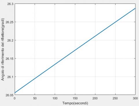
Figure 8. Reflector reference angle January 21st
When the real current intensity passing through the circuit is lower or higher than the reference current intensity, the switches open and/or close making sure that the sign of the voltage changes. This type of electronic control guarantees for the circuit that the circulating current is always the desired one.
To compare the current intensity of reference with the real one it is necessary that the model is able to estimate the effective current circulating. This calculation is carried out by implementing the written electrical equations, Eq. (7) and (8), written for both phases.
With reference to a linear Fresnel plant located at a latitude of 40 °N and with a receiver tube height of 3 meters, the results of some simulations referred to a typical day are shown below.
As an example, the results for the secondary rotation of the central reflector for January 21 are shown.
Figure 8 shows the trend of the reference angle,for an interval of 5 minutes, that ideally the panel should follow. The angle is determined by applying the law of motion described in Eq. (4).
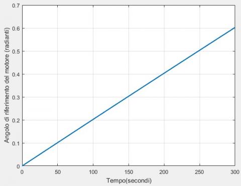
The rotation that the rotor should ideally follow, however, is kinematically linked to the rotation of the reflector by the transmission system according to the relations (12) and (13). In Figure 9 it is possible to observe the corresponding law of the reference motion of the rotor. The angle of the initial position has been set to 0°.
Figure 9. Reference angle of the rotor January 21st
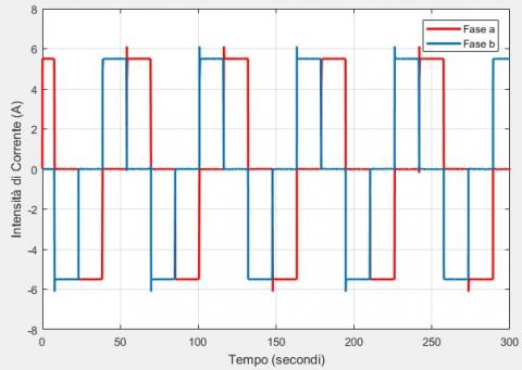
Figure 10. Current intensity circulating in the phases January 21st
Assuming that each step has an amplitude of 1.8° (0.0314 rad), the model generates the sequence of the reference currents and defines, in feedback, the temporal opening of the circuit-breakers so as to provide the voltage suitable to simulate the expected current trend. The actual circulating currents are determined by the implementation of the electrical equations to the mesh of the circuit and the results obtained are shown in Figure 10.
The current intensities have a square wave pattern, similar to that required to complete the steps. The alternation of the currents in the phases allows the motor to execute the steps. There are slight fluctuations caused by electrical inertia and above all mechanical ones.
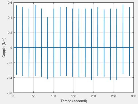
An important aspect to be evaluated is also represented by the torque values that the motor must be able to supply. We must take into account the fact, however, that the value obtained can be very variable according to the wind speed on the reflectors. The incidence of wind has not been taken into consideration in the discussion but, nevertheless, it is necessary to provide for the motor supplying about twice the maximum torque obtained. The calculated torque results are shown in Figure 11.
Figure 11. Torque supplied by the motor. January 21st
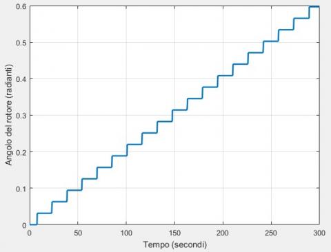
Figure 12. Rotor angle January 21st
The torque value is void for as long as no movement is required; peaks are reached in the instant the step is completed. Torque peaks, which have a maximum value of about 0.6 Nm, are necessary to overcome inertia forces.
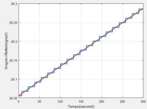
The actual angular position of the motor is shown in Figure 12. In Figure 13, instead, the real motion of the reflector superimposed on the theoretical motion is shown.
From the figure it is evident the error that is committed through the step movement. The maximum tracking error is approximately 0.02°.
Figure 13. Comparison of actual and desired reflector angle January 21st
Figure 14. Delivered torque January 21st
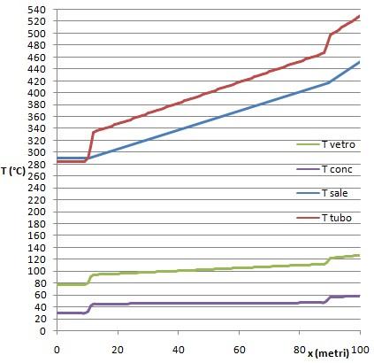
Figure 15. Temperature trends for December 21st
From the control point of view, the step response presents the trend of a feedback control system of the first order. In fact, with the electrical characteristics of the motor and the mechanical characteristics of the reflector under consideration, no settling oscillations of any kind are generated. Finally, in Figure 14, a zoom of the delivered torque is shown, which is cancelled with a time of about 3 seconds.
To highlight the gain, consequent to the use of primary biaxial tracking reflectors, the results obtained by applying the energy simulation model presented in [2] are reported, for a plant with a length of 100 meters and an absorber tube height of 5 m. The fluid used is a molten salt with a flow rate of 0.73 kg/s. Figure 15 shows, in particular, for December 21st at 12:00, the temperature trend of the glass tube, of the secondary concentrator, of the fluid and of the absorber tube.
From the Figure it is possible to distinguish three sections:
In the first section the temperature of the fluid and that of the pipe remain constant. This section of absorber, with a length of 10.4 m, is not affected by sunlight. The temperature of the tube is lower than that of the fluid since the molten salts, which are introduced at 290 °C, cool down.
In the second section the tube absorbs the radiative power concentrated by the reflectors and transfers thermal power to the fluid. The temperature of the pipe undergoes a sharp increase with consequent transfer of heat between the wall and the fluid that begins to increase its temperature in the direction of motion.
In the third section, of a length equal to the initial one, the thermal power that reaches the absorption system is approximately double compared to the second section. The primary reflectors with biaxial tracking, which in a classic linear Fresnel system would be unusable, direct further radiation on the final tube section. The slope of the fluid temperature curve increases and the pipe temperature undergoes a further sharp increase.
The efficiency obtained through the simulation was 65.1 %.
In the case, instead, of using primary reflectors with a single degree of freedom, what happens in the third section would not occur, and the second section would extend to the end of the collector. In classic Fresnel linear systems, the losses that occur at the beginning of the collector (in this case to the south) are not recovered in the final section. Under these conditions, plant efficiency would be 54.8 %.
The plant engineering solution with biaxial tracking reflectors proposed in the work would therefore involve, for the 100 m plant taken as a reference, an increase in efficiency of over 10 percentage points at the winter solstice.
The research involved the study of the handling system of a linear concentration Fresnel plant in which the reflectors at the ends are able to rotate around two axes. In this paper, the support structure of the terminal reflectors which allows them to rotate around two axes was presented. They must be able to rotate around the main axis directed in the longitudinal direction of the system, and around a secondary axis perpendicular to the first and which undergoes the primary rotation. In order to allow secondary motion, it is necessary for the servomotor to rotate solidly with the support on which the reflector is placed.
In this work, a dynamic study was then carried out to simulate the motion followed by the reflector. To do this, the coupling of the motors with the mechanical components was modelled. The control logic of the servomotors has been defined by solving the electrical equations applied to the windings and the cardinal equations of the dynamics that govern the motion of the mirrors. The analysis allowed the time trend that is actually followed by the reflector to be obtained.
The model made it possible to verify how the kinematic behaviour changes with the variation of the electrical quantities and the geometric characteristics of the reflector.
In the example case presented, the difference between the law of ideal motion and that actually followed by the reflector, and the values of the torque generated by the secondary servomotor are shown. The model presented, allowing assessment of the settling time and the oscillations around the equilibrium position after each step, is useful for a preliminary analysis that leads to the sizing of the various components.
The solution proposed in this work involves, a maximum yield increase of about 10 percentage points at the winter solstice for a plant of 100 m and height of the absorber of 5 m.
|
a |
solar azimuth, rad |
|
C |
torque, N.m |
|
d |
distance of the reflector from the projection of the tube on the ground, m |
|
h |
height of the tube, m |
|
i |
phase current, A |
|
I |
Nominal current, A |
|
J_p |
polar moment of inertia, kg.m2 |
|
k |
length of the unirradiated tube, m |
|
ke |
torque conversion factor, N.m.A-1 |
|
l |
length of reflector, m |
|
L |
phase inductance, H |
|
M |
mass of reflector, kg |
|
Nc |
number of pole-pairs |
|
r |
radius of gear wheel, m |
|
R |
electrical resistance, Ω |
|
s |
distance motor-reflector axis, m |
|
sp |
depth of reflector, m |
|
Tconc |
temperature of secondary reflector, °C |
|
Tsale |
temperature of molten salt, °C |
|
Ttubo |
temperature of absorber tube, °C |
|
Tvetro |
temperature of glass envelope, °C |
|
V |
phase voltage, V |
|
x, y, z |
spatial coordinates, m |
Greek symbols
|
α |
solar altitude, rad |
||
|
β |
tilt angle of mono-axial reflector, rad |
||
|
ΔL |
actuator linear displacement, m |
||
|
ΔV |
nominal voltage, V |
||
|
θ |
rotor angular position, rad |
||
|
θa |
azimuth angle of the normal to reflector, rad |
||
|
θα |
angular altitude of the normal to reflector, rad |
||
|
θP |
angle of primary rotation, degrees |
||
|
θq |
angle of secondary rotation, degrees |
||
|
ρ |
surface density, kg.m-3 |
||
|
ω ωP |
rotor angular speed, rad.s-1 reflector angular speed, rad.s-1 |
||
Subscripts
|
S |
sun |
|
a, b |
phases of motor |
[1] Abbas R, Munoz-Anton J, Valdes M, Martinez-Val JM. (2013). High concentration linear Fresnel reflectors. Energy Conversion and Management 72: 60-68. https://doi.org/10.1016/j.enconman.2013.01.039
[2] Cucumo M, Ferraro V, Kaliakatsos D, Mele M, Nicoletti F. (2016). Calculation model using finite-difference method for energy analysis in a concentrating solar plant with linear Fresnel reflectors. International Journal of Heat and Technology 34(2): 337-345. https://doi.org/10.18280/ijht.34S221
[3] Dellicompagni P, Franco J. (2019). Potential uses of a prototype linear Fresnel concentration system. Renewable Energy 136: 1044-1054. https://doi.org/10.1016/j.renene.2018.10.005
[4] Gabbrielli R, Castrataro P, Medico FD, Palo MD, Lenzo B. (2014). Levelized cost of heat for linear Fresnel concentrated solar systems. Energy Procedia 49: 1340-1349. https://doi.org/10.1016/j.egypro.2014.03.143
[5] Zhang X, Liu K, Shan X, Liu Y. (2014). Roll-to-roll embossing of optical linear Fresnel lens polymer film for solar concentration. Optics Express 22(S7): A1835-A1842. https://doi.org/10.1364/oe.22.0a1835
[6] Facão J, Oliveira AC. (2011). Numerical simulation of a trapezoidal cavity receiver for a linear Fresnel solar collector concentrator. Renewable Energy 36: 90-96. https://doi.org/10.1016/j.renene.2010.06.003
[7] Abbas R, Montes MJ, Piera M, Martinez-Val JM. (2012). Solar radiation concentration features in Linear Fresnel Reflector arrays. Energy Conversion and Management 54: 133-144. https://doi.org/10.1016/j.enconman.2011.10.010
[8] Cucumo M, Ferraro V, Kaliakatsos D, Mele M, Nicoletti F. (2017). Law of motion of reflectors for a linear Fresnel plant. International Journal of Heat and Technology 35(1): S78-S86. https://doi.org/10.18280/ijht.35Sp0111
[9] Cucumo M, Ferraro V, Kaliakatsos D, Mele M, Nicoletti F. (2018). Linear Fresnel Plant with primary reflectors movable around two axes. Advances in Modelling and Analysis A 55(3): 99-107. https://doi.org/10.18280/ama_a.550301