Saad Khadar | Abdellah Kouzou | Mohamed Monir Rezaoui | Ahmed Hafaifa
OPEN ACCESS
Open-End Winding Five-Phase Induction Motors (OEW-FPIM) can offer high degree of faults tolerance, reduced common-mode voltage and high torque density. These motors are placed in varying environments and conditions that ultimately reduces the motor efficiency and later leads to failure. This paper proposes a fault-tolerant sensorless sliding mode control based on a parameters estimation (stator resistance, stator inductance and mutual inductance between the stator phases and the rotor phases) of OEW-FPIM with the ability to run the system disturbance-free before and after a short circuit fault between turns. The proposed estimation scheme is intended to improve the system performance even in the fault condition. In addition, a sliding mode observer (SMO) is used to estimate the rotor speed. The simulation results of the proposed sensorless control under a short circuit fault between turns, wherein we demonstrate the effectiveness of the proposed strategy.
Open End Winding (OEW), Five-Phase Induction Motor (FPIM), fault-tolerant control, sliding mode control, Sliding Mode Observer (SMO), parameters estimation
Recently, multi-phase induction machines open-end winding topology has gained much attention for their use in applications where high reliability is required [1]. This is due to their intrinsic features like power splitting, higher torque density, equal power input from both sides of each winding, certain degree of fault tolerance, the possibility of the reduction of common mode voltage and the reducing of the output voltage distortion [2-4]. In spite of the previous advantages, these machines are subject to different types of faults due to various stresses during operating conditions. These faults can be divided according to the main components of the machine such as disorders of the stator, rotor, and bearings. Bell et al. [5] state that the stator winding failures are one of the major causes of motor failure. Also, it should be noted that the majority of the failures result from crash of winding insulation. The gradual deterioration process of the stator winding insulation is caused by a combination of thermal stresses (aging, overloading and cycling), mechanical stresses (coil movement and strikes from the rotor), electrical stresses and contamination [6-8].
On the other hand, stator winding consists of coils of insulated copper wire placed in the stator slots. An insulation breakdown between two adjacent turns in a coil for the same phase produces a stator winding fault. This kind of fault is called short circuit fault between turns (turn to turn). This fault cause a large circulating fault current in the shorted turns of the stator winding, leading to excessive heat generation in the shorted turns. This further degrades the insulation, and finally results to rapidly progress to more severe faults such as line-to-ground or line-to-line faults [8]. A detailed analysis of these types of fault can be found from Kwak’s research [9]. These faults can lead to the failure of complete phase, which may eventually lead to a catastrophic failure [10]. Consequently, the knowledge of machine behavior under short circuit fault between turns is extremely important from the standpoint of improved system design and fault tolerant control. Several modeling and simulation studies have been published, which can analyze the stator faults by different models such as the multi winding and multi-turns model [11]. Tallam et al. [12] presented a transient model using reference frame transformation theory. The data obtained with these models can provide useful information about the motors behavior under stator winding fault, but they require restrictive assumptions. These assumptions therefore lead to the omission of relevant information on the machine condition.
Based on the above discussion, this paper deals with a OEW-FPIM topology instead of the star connection topology, which is connected to dual two-level voltage inverters supplied by one DC source. Firstly, this paper presents a mathematical model by which behaviour of OEW-FPIM with short circuit between turns in the machine stator winding can be analyzed. The model is based on a theory of electromagnetic coupling of electrical circuits (the matrix coefficients of stator resistance (Rs), stator leakage inductance (ls), mutual inductance between stator phases (Mss) and mutual inductance stator-rotor (Msr), taking into account the changing motor parameter to calculate the number of turns in short-circuit [13]. After a modeling polyphase of the OEW-FPIM, it is desirable for the machine to continue operating under faulty conditions. For this purpose, a fault-tolerant sliding mode control strategy by parameter estimation (Rs, ls and Msr) is implemented. Although, this used control technique offers excellent performance, a better speed tracking response to the reference, robustness against disturbances and it is insensitive to uncertainties [14], but it requires the estimation of the motor parameters to ensure the robustness against the parameters variation (particularly, Rs, ls and Msr) which are used in machine modeling under stator winding fault. So, it is important the addition of parameters estimation algorithm in order to compensate for parameter variation effects, thus ensuring the machine ability to continue to operate under fault conditions until a safe stop. Therefore, a method for parallel estimation of Rs, ls and Msr using a Proportional-Integral (PI) controller has been investigated in this paper. This method is based on a simple algorithm capable of running in a low-cost microcontroller. In addition, to ensure a high-precision performance of the fault-tolerant sliding mode control, the accurate information obtained from the rotor flux and the rotor speed are more than necessary to achieve an accurate control and increase the reliability of the system. Usually, the controller receives the information of the motor speed from the speed sensors, such as tachometers, encoders, resolver, etc. However, practically these speed sensors are always accompanied by certain difficulties. To avoid the use of speed and flux sensors, a sliding mode observer is used in this work to estimate the flux and the speed, which has become the most used popular approach in ensuring an accurate estimation of the rotor speed and the rotor flux even in presence of stator faults and load torque disturbance, due to the design simplicity, the accuracy with a fast convergence and less computational time. The obtained simulation results confirm the clear efficacy of the proposed sensorless control strategy under healthy and faulty conditions.
2.1 Modeling of FPIM under stator winding fault
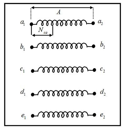
This paper studies the short circuit fault between turns in the stator winding of OEW-FPIM, which is shown in Figure 1, it is assumed that the short circuit is between 16 turns in the same phase, this means that approximately 10% of turns of A-phase are short circuited. Phase B, C, D and E have the same number of turns equal turns shorted of number the represents Nca the: where, Ns in phase (A).
Figure 1. Stator winding scheme with a short-circuits fault between 16 turns in first coil
This paper presents a method of polyphase modeling for OEW-FPIM. The method is based on the theory of electromagnetic coupling of electrical circuits, we get the new five phase model which represent the global model of the OEW-FPIM in the presence of stator winding faults, where the five-phase stator currents are determined according to the following equations [15]:
The rotor flux in the original reference frame can be given by:
\(\begin{align} & \frac{d{{i}_{sa}}}{dt}={{U}_{SA}}+{{A}_{1}}{{i}_{sa}}+{{A}_{2}}{{i}_{sb}}+{{A}_{3}}{{i}_{sc}}+{{A}_{4}}{{i}_{sd}}+{{A}_{5}}{{i}_{se}}+k{{f}_{sa}}f_{sb}^{2}f_{sc}^{2}f_{sd}^{2}f_{se}^{2}\left( G{{\varphi }_{sa}}+{{G}_{1}}{{\varphi }_{sb}}-{{G}_{2}}{{\varphi }_{sc}}+{{G}_{1}}{{\varphi }_{sd}}-{{G}_{2}}{{\varphi }_{se}} \right) \\ & \frac{d{{i}_{sb}}}{dt}={{U}_{SB}}+{{B}_{1}}{{i}_{sa}}+{{B}_{2}}{{i}_{sb}}+{{B}_{3}}{{i}_{sc}}+{{B}_{4}}{{i}_{sd}}+{{B}_{5}}{{i}_{se}}+kf_{sa}^{2}f_{sb}^{{}}f_{sc}^{2}f_{sd}^{2}f_{se}^{2}\left( -{{G}_{2}}{{\varphi }_{sa}}+G{{\varphi }_{sb}}+{{G}_{1}}{{\varphi }_{sc}}-{{G}_{2}}{{\varphi }_{sd}}+{{G}_{1}}{{\varphi }_{se}} \right) \\ & \frac{d{{i}_{sc}}}{dt}={{U}_{SC}}+{{C}_{1}}{{i}_{sa}}+{{C}_{2}}{{i}_{sb}}+{{C}_{3}}{{i}_{sc}}+{{C}_{4}}{{i}_{sd}}+{{C}_{5}}{{i}_{se}}+kf_{sa}^{2}f_{sb}^{2}f_{sc}^{{}}f_{sd}^{2}f_{se}^{2}\left( {{G}_{1}}{{\varphi }_{sa}}-{{G}_{2}}{{\varphi }_{sb}}+G{{\varphi }_{sc}}+{{G}_{1}}{{\varphi }_{sd}}-{{G}_{2}}{{\varphi }_{se}} \right) \\ & \frac{d{{i}_{sd}}}{dt}={{U}_{SD}}+{{D}_{1}}{{i}_{sa}}+{{D}_{2}}{{i}_{sb}}+{{D}_{3}}{{i}_{sc}}+{{D}_{4}}{{i}_{sd}}+{{D}_{5}}{{i}_{se}}+kf_{sa}^{2}f_{sb}^{2}f_{sc}^{2}f_{sd}^{{}}f_{se}^{2}\left( -{{G}_{2}}{{\varphi }_{sa}}+{{G}_{1}}{{\varphi }_{sb}}-{{G}_{2}}{{\varphi }_{sc}}+{{G}_{{}}}{{\varphi }_{sd}}+{{G}_{1}}{{\varphi }_{se}} \right) \\ & \frac{d{{i}_{se}}}{dt}={{U}_{SE}}+{{E}_{1}}{{i}_{sa}}+{{E}_{2}}{{i}_{sb}}+{{E}_{3}}{{i}_{sc}}+{{E}_{4}}{{i}_{sd}}+{{E}_{5}}{{i}_{se}}+kf_{sa}^{2}f_{sb}^{2}f_{sc}^{2}f_{sd}^{2}f_{se}^{{}}\left( {{G}_{1}}{{\varphi }_{sa}}-{{G}_{2}}{{\varphi }_{sb}}+{{G}_{1}}{{\varphi }_{sc}}-{{G}_{2}}{{\varphi }_{sd}}+{{G}_{{}}}{{\varphi }_{se}} \right) \\\end{align}\) (1)
The constants ($U_{S A}, U_{S B}, U_{S C}, U_{S D}, U_{S E}$) are defined as follows:
\(\begin{align} & \frac{d{{\varphi }_{ra}}}{dt}=\lambda \left( {{f}_{sa}}{{i}_{sa}}-\frac{{{f}_{sb}}}{2}{{i}_{sb}}-\frac{{{f}_{sc}}}{2}{{i}_{sc}}-\frac{{{f}_{sd}}}{2}{{i}_{sd}}-\frac{{{f}_{se}}}{2}{{i}_{se}} \right)-{{k}_{A1}}{{\varphi }_{ra}}-{{k}_{A2}}{{\varphi }_{rb}}-{{k}_{A3}}{{\varphi }_{rc}}-{{k}_{A2}}{{\varphi }_{rd}}-{{k}_{A3}}{{\varphi }_{re}} \\ & \frac{d{{\varphi }_{rb}}}{dt}=\lambda \left( -\frac{{{f}_{sa}}}{2}{{i}_{sa}}+{{f}_{sb}}{{i}_{sb}}-\frac{{{f}_{sc}}}{2}{{i}_{sc}}-\frac{{{f}_{sd}}}{2}{{i}_{sd}}-\frac{{{f}_{se}}}{2}{{i}_{se}} \right)-{{k}_{A3}}{{\varphi }_{ra}}-{{k}_{A1}}{{\varphi }_{rb}}-{{k}_{A2}}{{\varphi }_{rc}}-{{k}_{A3}}{{\varphi }_{rd}}-{{k}_{A2}}{{\varphi }_{re}} \\ & \frac{d{{\varphi }_{rc}}}{dt}=\lambda \left( -\frac{{{f}_{sa}}}{2}{{i}_{sa}}-\frac{{{f}_{sb}}}{2}{{i}_{sb}}+{{f}_{sc}}{{i}_{sc}}-\frac{{{f}_{sd}}}{2}{{i}_{sd}}-\frac{{{f}_{se}}}{2}{{i}_{se}} \right)-{{k}_{A2}}{{\varphi }_{ra}}-{{k}_{A3}}{{\varphi }_{rb}}-{{k}_{A1}}{{\varphi }_{rc}}-{{k}_{A2}}{{\varphi }_{rd}}-{{A}_{3}}{{\varphi }_{re}} \\ & \frac{d{{\varphi }_{rd}}}{dt}=\lambda \left( -\frac{{{f}_{sa}}}{2}{{i}_{sa}}-\frac{{{f}_{sb}}}{2}{{i}_{sb}}-\frac{{{f}_{sc}}}{2}{{i}_{sc}}+{{f}_{sd}}{{i}_{sd}}-\frac{{{f}_{se}}}{2}{{i}_{se}} \right)-{{k}_{A3}}{{\varphi }_{ra}}-{{k}_{A2}}{{\varphi }_{rb}}-{{k}_{A3}}{{\varphi }_{rc}}-{{k}_{A1}}{{\varphi }_{rd}}-{{k}_{A2}}{{\varphi }_{re}} \\ & \frac{d{{\varphi }_{re}}}{dt}=\lambda \left( -\frac{{{f}_{sa}}}{2}{{i}_{sa}}-\frac{{{f}_{sb}}}{2}{{i}_{sb}}-\frac{{{f}_{sc}}}{2}{{i}_{sc}}-\frac{{{f}_{sd}}}{2}{{i}_{sd}}+{{f}_{se}}{{i}_{se}} \right)-{{k}_{A2}}{{\varphi }_{ra}}-{{k}_{A3}}{{\varphi }_{rb}}-{{k}_{A2}}{{\varphi }_{rc}}-{{k}_{A3}}{{\varphi }_{rd}}-{{k}_{A1}}{{\varphi }_{re}} \\\end{align}\) (2)
where
\(\begin{align} & {{U}_{SA}}={{d}_{1}}f_{sb}^{2}f_{sc}^{2}f_{sd}^{2}f_{se}^{2}{{V}_{sa}}+{{d}_{2}}{{f}_{sa}}f_{sb}^{{}}f_{sc}^{{}}f_{sd}^{2}f_{se}^{{}}{{V}_{sb}}+{{d}_{2}}{{f}_{sa}}f_{sb}^{2}f_{sc}^{{}}f_{sd}^{{}}f_{se}^{{}}{{V}_{sc}}+{{d}_{2}}{{f}_{sa}}f_{sb}^{{}}f_{sc}^{{}}f_{sd}^{{}}f_{se}^{2}{{V}_{sd}}+{{d}_{2}}{{f}_{sa}}f_{sb}^{{}}f_{sc}^{2}f_{sd}^{{}}f_{se}^{{}}{{V}_{se}} \\ & {{U}_{SB}}={{d}_{2}}{{f}_{sa}}f_{sb}^{{}}f_{sc}^{{}}f_{sd}^{2}f_{se}^{{}}{{V}_{sa}}+{{d}_{1}}f_{sa}^{2}f_{sc}^{2}f_{sd}^{2}f_{se}^{2}{{V}_{sb}}+{{d}_{2}}f_{sa}^{2}f_{sb}^{{}}f_{sc}^{{}}f_{sd}^{{}}f_{se}^{2}{{V}_{sc}}+{{d}_{2}}{{f}_{sa}}f_{sb}^{{}}f_{sc}^{2}f_{sd}^{{}}f_{se}^{{}}{{V}_{sd}}+{{d}_{2}}f_{sa}^{2}f_{sb}^{{}}f_{sc}^{{}}f_{sd}^{{}}f_{se}^{{}}{{V}_{se}} \\ & {{U}_{SC}}={{d}_{2}}{{f}_{sa}}f_{sb}^{2}f_{sc}^{{}}f_{sd}^{{}}f_{se}^{{}}{{V}_{sa}}+{{d}_{2}}{{f}_{sa}}f_{sb}^{{}}f_{sc}^{{}}f_{sd}^{{}}f_{se}^{2}{{V}_{sb}}+{{d}_{1}}f_{sa}^{2}f_{sc}^{2}f_{sd}^{2}f_{se}^{2}{{V}_{sc}}+{{d}_{2}}f_{sa}^{2}f_{sb}^{{}}f_{sc}^{{}}f_{sd}^{{}}f_{se}^{{}}{{V}_{sd}}+{{d}_{2}}f_{sa}^{{}}f_{sb}^{{}}f_{sc}^{{}}f_{sd}^{2}f_{se}^{{}}{{V}_{se}} \\ & {{U}_{SD}}={{d}_{2}}{{f}_{sa}}f_{sb}^{{}}f_{sc}^{{}}f_{sd}^{{}}f_{se}^{2}{{V}_{sa}}+{{d}_{2}}{{f}_{sa}}f_{sb}^{{}}f_{sc}^{2}f_{sd}^{{}}f_{se}^{{}}{{V}_{sb}}+{{d}_{2}}f_{sa}^{2}f_{sb}^{{}}f_{sc}^{{}}f_{sd}^{{}}f_{se}^{{}}{{V}_{sc}}+{{d}_{1}}f_{sa}^{2}f_{sc}^{2}f_{sd}^{2}f_{se}^{2}{{V}_{sd}}+{{d}_{2}}f_{sa}^{{}}f_{sb}^{2}f_{sc}^{{}}f_{sd}^{{}}f_{se}^{{}}{{V}_{se}} \\ & {{U}_{SE}}={{d}_{2}}{{f}_{sa}}f_{sb}^{{}}f_{sc}^{2}f_{sd}^{{}}f_{se}^{{}}{{V}_{sa}}+{{d}_{2}}f_{sa}^{2}f_{sb}^{{}}f_{sc}^{{}}f_{sd}^{{}}f_{se}^{{}}{{V}_{sb}}+{{d}_{2}}{{f}_{sa}}f_{sb}^{{}}f_{sc}^{{}}f_{sd}^{2}f_{se}^{{}}{{V}_{sc}}+{{d}_{2}}{{f}_{sa}}f_{sb}^{2}f_{sc}^{{}}f_{sd}^{{}}f_{se}^{{}}{{V}_{sd}}+{{d}_{1}}f_{sa}^{2}f_{sc}^{2}f_{sd}^{2}f_{se}^{2}{{V}_{se}} \\\end{align}\) (3)
The mechanical equation of rotor motion is given as follows:
$J \frac{d \Omega}{d t}+F \Omega=T_{e}-T_{L}$ (4)
The electromagnetic torque can be found using the stator current and rotor flux as well as the motor parameters and it is deduced from equation:
$T_{e}=n_{p} \frac{M_{s r}}{L_{r}}\left(\left[i_{s}\right] \wedge\left[\varphi_{r}\right]\right)$ (5)
where, $J, n_{p}, M_{r r}, l_{r}, R_{r}$ and F are the rotor resistance, the rotor leakage inductance, the mutual inductance rotor-rotor, the number of pairs of poles, the moment of inertia of the motor and the viscous friction coefficient, respectively.
2.2 Open Winding inverter configuration with one dc source
This paper mainly discusses the open-end winding five-phase induction motor supplied by a dual inverter with one DC source [15, 16]. In this configuration, the common mode voltage is forced to zero because of the connection path between the two inverters [17]. The power circuit configuration consists of the dual five-phase voltage source inverter and the five phase induction motor with open-end stator windings. The dual inverters and their elements are identified by indices 1 and 2. Inverter 1 is connected to machine stator phases terminal of a1, b1, c1, d1, e1, and inverter 2 is connected to machine stator phases terminal of a2, b2, c2, d2, e2. Each inverter branch consists of two power electronics switches operated alternately. The switching state for inverter 1 are defined as Sa, Sb, Sc, Sd, Se and the switching state of inverter 2 are defined as SA, SB, SC, SD, SE.
3.1 The sliding mode control based on Field-Oriented control
The method of sliding mode control associated to the Field-Oriented Control (FOC) has been applied for the control of the OEW-FPIM. The main objective of the FOC strategy is to independently control the electromagnetic torque and the rotor flux. The control strategy used consist to maintain the quadrature component of the flux null and the direct flux equals to the reference, and can be described as follows [18, 19]:
$\varphi_{r d}=\varphi_{r}$
$\varphi_{r q}=0$ (6)
The FOC strategy is based on the mathematical model of the FPIM formulated in the synchronous reference frame (d-q-x-y) can be presented as follows [1]:
$\left\{\begin{array}{c}\frac{d i_{s d}}{d t}=\left(\frac{M_{s r}^{2} R_{r}+R_{s} L_{r}^{2}}{\sigma L_{s} L_{r}^{2}}\right) i_{s d}+\omega i_{s q}+\left(\frac{M_{s r} R_{r}}{\sigma L_{s} L_{r}}\right) \varphi_{r}+\frac{1}{\sigma L_{s}} V_{s d} \\ \frac{d i_{s q}}{d t}=\left(\frac{M_{s r}^{2} R_{r}+R_{s} L_{r}^{2}}{\sigma L_{s} L_{r}^{2}}\right) i_{s q}-\omega i_{s d}+\left(\frac{M_{s r} R_{r}}{\sigma L_{s} L_{r}}\right) \varphi_{r}+\frac{1}{\sigma L_{s}} V_{s q} \\ \frac{d i_{s x}}{d t}=-\frac{R_{s}}{l_{s}} i_{s r}+\frac{1}{l_{s}} V_{s x} \\ \frac{d i_{s y}}{d t}=-\frac{R_{s}}{l_{s}} i_{s y}+\frac{1}{l_{s}} V_{s y}\end{array}\right.$ (7)
In the synchronous reference, two orthogonal frames called d-q and x-y are used. Where, the components d-q are responsible for developing the fluxes and the torque, while the remaining x-y components generate the machine losses. Applying the (6), the torque equation become analogous to the DC machine [19] as described by:
$T_{e}=\frac{n_{p} M_{s r}}{J L_{r}} \varphi_{r} i_{s q}$ (8)
The slip relation is given by:
$\omega_{s l}=\frac{n_{p} M_{s r}}{\varphi_{r} T_{r}} i_{s q}$ (9)
with: $\sigma=1-\frac{M_{s r}}{L_{s} L_{r}}$
The sliding mode control strategy is developed to solve the disadvantage of other design of non-linear control. This strategy adjust feedback by previously defining a surface, so that the system which is controlled will be forced to that surface, then the behaviour of the system slides to the desired equilibrium point. The main feature of this strategy is that we only need to drive the error to a switching surface. When the system is in the sliding mode, the system behaviour is not affected by any modelling uncertainties and/or disturbances [20]. The control strategy includes two terms, the first for the exact linearization, the second discontinuous one for the system stability are defined as [8]:
$X=X_{e q}+X_{m}$ (10)
with: $X_{m}=K_{m} \operatorname{sgn}(S(X))$
Here X is the control vector, Xeq is the equivalent control vector, Xm is given to guarantee the attractively of the variable to be controlled towards the commutation surface (the correction factor). Km is a constant, being the maximal value of the controller output and sgn is the sign function. The control strategy design includes two steps:
The first step consists in defining the sliding surfaces and the dynamics of the variables to be controlled such as the rotor speed and the rotor flux, where the dynamics of the variables is presented by their corresponding derivatives, which are expressed as follows:
$\left\{\begin{array}{l}s_{\omega}=\omega^{*}-\omega \\ s_{\varphi}=\varphi_{r}^{*}-\varphi_{r} \\ \dot{s}_{\omega}=\dot{\omega}^{*}-\dot{\omega} \\ \dot{s}_{\varphi}=\dot{\varphi}_{r}^{*}-\dot{\varphi}_{r}\end{array}\right.$ (11)
By using the mechanical equations defined in the (7) and the derivative of the (11), the derivative of the sliding surface can be calculated as [21]:
$\left\{\begin{array}{l} \dot{s}_{\omega}=\dot{\omega}^{*}-\frac{\frac{n_{p} M_{s r}}{J L_{r}} i_{s q} \varphi_{r}-F \omega-T_{L}}{J} \\ \dot{s}_{\varphi}=\dot{\varphi}_{r}^{*}+\frac{\varphi_{r}-M_{s r} i_{s d}}{T_{r}}\end{array}\right.$ (12)
The output signal of the stator current reference are defined by the following expressions:
$\left\{\begin{array}{l}i_{s q m}=k_{i s q} \operatorname{sgn}\left(\mathrm{s}_{\omega}\right) \\ i_{s q e q}=\frac{L_{r}\left(J \dot{\omega}^{*}+F \omega+T_{L}\right)}{n_{p} M_{s r} \varphi_{r}} \\ i_{s q}^{*}=i_{s q e q}+i_{i s q m}\end{array}\right.$ (13)
$\left\{\begin{array}{l}i_{s d m}=k_{i s d} \operatorname{sgn}\left(s_{\varphi}\right) \\ i_{s d e q}=\frac{T_{r} \varphi_{r}}{M_{s r}}+\frac{\varphi_{r}}{M_{s r}} \\ i_{s d}^{*}=i_{s d m}+i_{s d e q}\end{array}\right.$ (14)
This reference current will be used in the following step for constructing the control law. Indeed, in the second step, the control law $V_{s d}^{*}$ and $V_{S q}^{*}$ of the whole system are determined, where the two new sliding surfaces of the current stator components along d-q axis, which is determined by the following system of equations:
$\left\{\begin{array}{c}s_{s_{s d}}=i_{s d}^{*}-i_{s d} \\ s_{s_{s_{g}}}=i_{s q}^{*}-i_{s q} \\ \dot{s}_{i_{s d}}=\frac{d i_{s d}^{*}}{d t}-\frac{d i_{s d}}{d t} \\ \dot{s}_{i_{s q}}=\frac{d i_{s q}^{*}}{d t}-\frac{d i_{s q}}{d t}\end{array}\right.$ (15)
By using the (14) and after some algebraic operations, the derivative of the sliding surface can be calculated as:
$\left\{\begin{array}{l}\dot{s}_{i_{g_{q}}}=\frac{d i_{s d}^{*}}{d t}-\frac{V_{s q}-R_{s} i_{s q}-\omega_{k}\left(L_{s} i_{s d}+\varphi_{r}\right)}{L_{s}} \\ \dot{s}_{i_{s, d}}=\frac{d i_{s q}^{*}}{d t}-\frac{V_{s d}-R_{s_{s d}} i_{s d}+\omega_{k}\left[L_{s} i_{s q}+\frac{L_{r}\left(\omega_{k}-\omega\right) \varphi_{r}}{R_{r}}\right]}{L_{s}}\end{array}\right.$ (16)
Finally, the stator tensions reference are obtained by the following expressions:
$\left\{\begin{array}{l}V_{s q m}=k_{v s q} \operatorname{sgn}\left(s_{s_{s q}}\right) \\ V_{s q e q}=L_{s} \frac{d i_{s q}^{*}}{d t}+R_{s} i_{s q}+\omega_{k}\left(L_{s} i_{s d}+\varphi_{r}\right) \\ V_{s q}^{*}=V_{s q e q}+V_{s q m}\end{array}\right.$ (17)
$\left\{\begin{array}{l}V_{s d m}=k_{v s d} \operatorname{sgn}\left(s_{i_{s d}}\right) \\ V_{s d e q}=L_{s} \frac{d i_{s d}^{*}}{d t}+R_{s} i_{s d}-\omega_{k}\left[L_{s} i_{s q}+\frac{L_{r}\left(\omega_{k}-\omega\right) \varphi_{r}}{R_{r}}\right] \\ V_{s d}^{*}=V_{s d e q}+V_{s d m}\end{array}\right.$ (18)
To ensure the control stability, the gains kisd, kisq, kvsd and kvsq should be taken positive by selecting the appropriate values, where: $\omega_{k}=\frac{M_{s r} i_{s q}}{T_{r} \varphi_{r}}+\omega$
3.2 The Sliding Mode Observer (SMO)
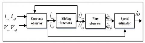
The sliding mode observer (SMO) presented in this paper, is the original one proposed by Chiheb et al. [22], its basic principal is shown in Figure 2. This structure does not require knowledge speed, the design simplicity, the accuracy with a fast convergence and less computational time, unlike other observers. The motor model are defined in the stationary reference frame as follows:
Figure 2. The block diagram of the SMO model
$\left[\begin{array}{c}\frac{d i_{s \alpha}}{d t} \\ \frac{d i_{s \beta}}{d t}\end{array}\right]=\eta\left(\begin{array}{cc}\beta_{r} & -\omega \\ -\omega & \beta_{r}\end{array}\right)\left[\begin{array}{c}\varphi_{r \alpha} \\ \varphi_{r \beta}\end{array}\right]-\gamma\left[\begin{array}{c}i_{s \alpha} \\ i_{s \beta}\end{array}\right]+\delta\left[\begin{array}{c}V_{s \alpha} \\ V_{s \beta}\end{array}\right]$ (19)
$\left[\begin{array}{c}\frac{d \varphi_{r \alpha}}{d t} \\ \frac{d \varphi_{r \beta}}{d t}\end{array}\right]=\left(\begin{array}{cc}-\beta_{r} & -\omega \\ \omega & -\beta_{r}\end{array}\right)\left[\begin{array}{c}\varphi_{r \alpha} \\ \varphi_{r \beta}\end{array}\right]+\beta_{r} M_{s r}\left[\begin{array}{c}i_{s \alpha} \\ i_{s \beta}\end{array}\right]$ (20)
The equations of the stator currents and the rotor flux for the SMO model can be presented as follows:
$\left[\begin{array}{c}\frac{d \hat{\imath}_{s \alpha}}{d t} \\ \frac{d \hat{\imath}_{s \beta}}{d t}\end{array}\right]=\eta\left[\begin{array}{l}U_{r \alpha} \\ U_{r \beta}\end{array}\right]-\gamma\left[\begin{array}{l}\hat{l}_{s \alpha} \\ \hat{l}_{s \beta}\end{array}\right]+\delta\left[\begin{array}{l}V_{s \alpha} \\ V_{s \beta}\end{array}\right]$ (21)
$\left[\begin{array}{c}\frac{d \hat{\varphi}_{r \alpha}}{d t} \\ \frac{d \hat{\varphi}_{r \beta}}{d t}\end{array}\right]=\left[\begin{array}{l}U_{r \alpha} \\ U_{r \beta}\end{array}\right]+\beta_{r} M_{s r}\left[\begin{array}{c}i_{s \alpha} \\ i_{s \beta}\end{array}\right]$ (22)
The Urα and Urβ are defined by:
$U_{r \alpha}=-k'' \operatorname{sign}\left(S_{s \alpha}\right)$
$U_{r \beta}=-k^{\prime \prime \prime} \operatorname{sign}\left(S_{s \beta}\right)$ (23)
with:
$S_{s \alpha}=\hat{\imath}_{s \alpha}-i_{s \alpha}, S_{s \beta}=\hat{\imath}_{s \beta}-i_{s \beta}$$\eta=\frac{M_{S T}}{\sigma L_{S} L_{r}}$,
$\gamma=\frac{R_{s}}{\sigma L_{s}}+\frac{R_{r} M_{s r}^{2}}{\sigma L_{s} L_{r}^{2}}, \delta=\frac{1}{\sigma L_{s}}, \beta_{r}=\frac{1}{T_{r}}$
From the equivalent control concept [23] assuming the observed currents $\hat{\imath}_{S \alpha}$ and $\hat{\imath}_{s \beta}$ must converge to those measured, from the (21) and (23), the following equation is obtained:
$\left[\begin{array}{c}U_{r \alpha}^{e q} \\ U_{r \beta}^{e q}\end{array}\right]=\left(\begin{array}{cc}\beta_{r} & \hat{\omega} \\ -\hat{\omega} & \beta_{r}\end{array}\right)\left[\begin{array}{c}\hat{\varphi}_{r \alpha} \\ \hat{\varphi}_{r \beta}\end{array}\right]$ (24)
On the same time by reorganizing the (24), it can be rewritten as follows:
$\left[\begin{array}{c}U_{r \alpha}^{e q} \\ U_{r \beta}^{e q}\end{array}\right]=\left(\begin{array}{cc}\hat{\varphi}_{r \alpha} & \hat{\varphi}_{r \beta} \\ \hat{\varphi}_{r \beta} & -\hat{\varphi}_{r \alpha}\end{array}\right)\left[\begin{array}{l}\hat{\beta}_{r} \\ \widehat{\omega}\end{array}\right]$ (25)
By using the (24) and (25), the $\widehat{\omega}$ and $\widehat{\beta_{r}}$ can be expressed as follows:
$\left[\begin{array}{c}\hat{\beta}_{r} \\ \widehat{\omega}\end{array}\right]=\frac{1}{\left|\widehat{\varphi}_{r \alpha}^{2}+\widehat{\varphi}_{r \beta}^{2}\right|}\left(\begin{array}{cc}-\widehat{\varphi}_{r \alpha} & -\hat{\varphi}_{r \beta} \\ -\hat{\varphi}_{r \beta} & \hat{\varphi}_{r \alpha}\end{array}\right)\left[\begin{array}{c}U_{r \alpha}^{e q} \\ U_{r \beta}^{e q}\end{array}\right]$ (26)
The estimation value of the rotor speed is found by:
$\widehat{\omega}=\frac{1}{\left|\widehat{\varphi}_{r \alpha}^{2}+\widehat{\varphi}_{r \beta}^{2}\right|}\left(\widehat{\varphi}_{r \alpha} U_{r \alpha}^{e q}-\widehat{\varphi}_{r \beta} U_{r \alpha}^{e q}\right)$ (27)
3.3 Motor parameters estimation
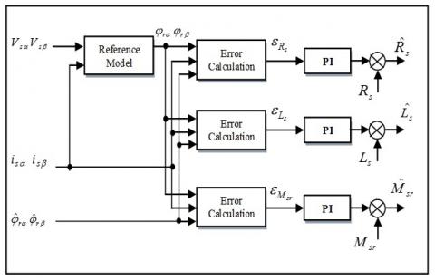
Figure 3 shows block diagram of the proposed parallel motor parameters estimation. The motor parameter changes due to the machine modeling with short circuit fault between turns. The control system may become unstable if the motor parameter values used in the controller differs from that of the machine parameters. So, the compensation for the effect of this variation then becomes necessary. Also, the sliding mode control can be made more reliable if the motor parameters are estimated. Therefore, this paper presents a estimation method of the (Rs), the (Ls) and the (Msr) in parallel using PI controller to compensate the changes in parameters during operation of machine.
Figure 3. The block diagram of the motor parameters estimation
3.3.1 Stator resistance estimation
It is well known that the motor stator resistance varies during the motor operation state due mainly to the variation of the stator windings temperature [1]. Therefore, to ensure the on-line estimation of the Rs. One may use a simple PI controller to achieve this objective. The rotor flux error between the flux model described by (20) and the observer described by (22) can be considered to be caused by the Rs variation. The error quantity is given by:
$\varepsilon_{R_{S}}=i_{s \alpha}\left(\varphi_{r \alpha}-\hat{\varphi}_{r \alpha}\right)+i_{s \beta}\left(\varphi_{r \beta}-\hat{\varphi}_{r \beta}\right)$ (28)
The error quantity in the rotor flux is used as an input to the PI controller. The output of the PI controller is the required change of the Rs, it is continuously added to the previously stator resistance. The Rs is on-line estimated by [1]:
$\hat{R}_{s}=R_{s}+K_{P R_{s}} \varepsilon_{R_{s}}+K_{I R_{s}} \int \varepsilon_{R_{s}} d t$ (29)
where, $K_{P R_{S}}$ and $K_{I R_{S}}$ are the proportional and the integral parameters of the PI resistance controller.
3.3.2 Stator inductance estimation
Similarly, by using the flux model in (20), and by using measurements of the stator currents in the stationary reference frame, we used a PI controller to estimate stator inductance. The adaptation signal is used as an input to the PI controller by:
$\varepsilon_{L_{s}}=\left(\varphi_{r \alpha}-\hat{\varphi}_{r \alpha}\right)\left(M_{s r} i_{s \alpha}-\hat{\varphi}_{r \alpha}\right)$$+\left(\varphi_{r \beta}-\hat{\varphi}_{r \beta}\right)\left(M_{s r} i_{s \beta}-\hat{\varphi}_{r \beta}\right)$ (30)
According to the (30), the Ls can be estimated by:
$\hat{L}_{s}=L_{s}+K_{P L_{s}} \varepsilon_{L_{s}}+K_{L_{s}} \int \varepsilon_{L_{s}} d t$ (31)
where, $K_{P L_{S}}$ and $\mathrm{K}_{I L_{S}}$ are the proportional and integral gains of the PI inductance controller.
3.3.3 Mutual inductance Stator-Rotor estimation
Having estimated the two most critical parameters Rs and Ls. An estimator has been designed to estimate the change in the mutual inductance stator-rotor. Msr may be corrected by referring to the magnitude deviation. The error quantity in the magnitude of the rotor flux vector and if a change is detected, a corresponding change in the Msr is made.
$\varepsilon_{M_{s r}}=\sqrt{\varphi_{r \alpha}^{2}+\varphi_{r \beta}^{2}}$$-\sqrt{\hat{\varphi}_{r \alpha}^{2}+\hat{\varphi}_{r \beta}^{2}}$ (32)
The equation for the $M_{s r}$ estimation is obtained by:
$\hat{M}_{s r}=M_{s r}+K_{P M_{s r}} \varepsilon_{M_{s r}}+K_{I M_{s r}} \int \varepsilon_{M_{s r}} d t$ (33)
where, $K_{P M_{S T}}$ and $K_{I M_{S r}}$ are the proportional and integral gains of the PI mutual controller.
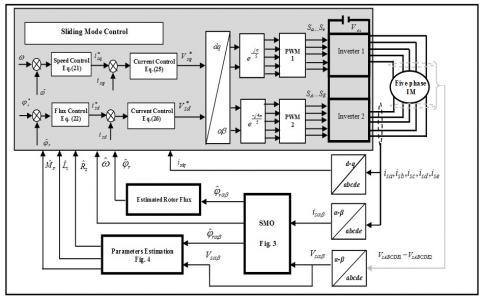
The block diagram of the proposed fault-tolerant sliding mode control using a motor parameters estimation for OEW-FPIM based on the SMO is shown in Figure 4. The control scheme allows to eliminate the speed sensor, where the real speed signal is replaced by the estimated one. In order to validate the effectiveness of the proposed control scheme, a some numerical simulation have been conducted by using MATLAB/SIMULINK. The control system has been tested in several operating conditions such as the following: healthy operation, faulty operation and fault-tolerant operation. The parameters of the studied OEW-FPIM for simulation are listed in the following: Rs=10Ω, Rr=6.3Ω, Ls=0.4642H, Lr=0.4642H, Msr=0.4212H, J=0.02 Kg⁄m2, F=0 N.m.s. The reference rotor flux used is 1 Wb.
Figure 4. The basic scheme for the fault-tolerant sliding mode control of OEW-FPIM based on SMO and motor parameter estimation
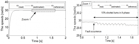
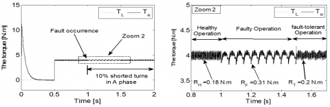
In order to verify the effectiveness and the strong robustness to fault of the proposed sliding mode control strategy based on motor parameters estimator from healthy operation to fault-tolerant operation at reference speed of 30 rad/sec and a 4 N.m of the load torque is applied during the test at 0.5 sec, the control system performance with and without the motor parameters estimation are compared. Simulation results are given in Figures. 5 to 9, respectively illustrating the speeds, the electromagnetic torque, the rotor flux, the five phase stator currents and the motor parameters under the short-circuit fault which touch 10% of the turns of the first phase (A), that is to say 16 turns of the coil are short circuited. During the Fault-Tolerant operation of the OEW-FPIM, the 10 % turn to turn short circuit fault occurs at 1 sec, and then the motor parameters estimator is activated at 1.5sec. Figure 5 presents the responses of the reference, real and estimated speed, it can be observed that the real and estimated speed values decreases slightly and oscillates around the 29.9 rad/sec after the fault occurrence. The appearance of these oscillations is directly related to the existence of a residual asymmetry in the motor stator circuit, when the motor parameters estimation is activated at t=1.5, it is clear that the real rotor speed is capable to return to the estimated rotor speed value quickly with the oscillation is negligible as its amplitude is less than one percent (see Zoom 1). Figure 6 shows the electromagnetic torque and the load torque, before and after the fault appearance without and with the motor parameters estimator. It can be seen that under the healthy condition, the torque fluctuations is 0.18 N.m. When the 10% short circuit fault occur, the torque fluctuations is 0.31 N.m. In fact, these cause fluctuations of the rotor speed, which generates acoustic noise and thus, an abnormal operation of the motor. When the motor parameters estimation is activated at t=1.5 or after the control program switches to the fault-tolerant operation, the torque fluctuations is relatively low is 0.2 N.m. Thus, the torque fluctuations is the same in the healthy operation.
Figure 5. The real, estimated and reference speed
Figure 6. The electromagnetic torque and the load torque
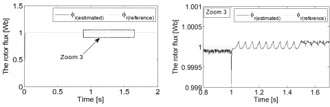
Figure 7. The reference and estimated rotor flux
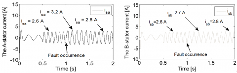
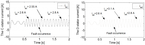
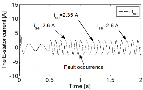
Figure 7 shows the reference and estimated rotor flux. It can be seen that the short circuit fault between turns of the same coil introduced some small fluctuations in the rotor flux. As soon as the motor parameters estimation is enabled, the rotor flux converge toward the desired value with fluctuations slightly. Figure 9 shows the measured five phase stator currents behavior when 10% of short-circuited. Initially, before the occurrence of the stator winding faults, both of these currents are balanced. However, with fault occurrence (t=1sec), the stator currents becomes unbalanced. The A-phase current becomes the largest one. This increase is related to the number of coils in short-circuit. This is obviously the simultaneous decrease of resistance and the inductances. However, the D-phase current amplitude is enlarged, whose amplitude is bigger than B,C, E phase currents. but when the motor parameters estimation is activated at t=1.5, the five-phase stator currents is similar to measured ones in healthy case and they have equal magnitudes.
Figure 8. The measured five-phase stator currents
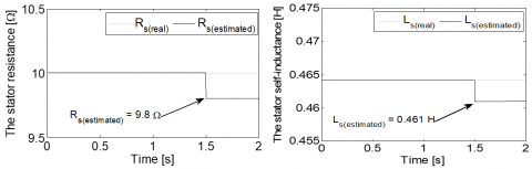
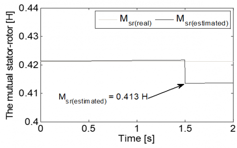
Figure9. The motor parameters variations
Figure 9 shows the real and estimated motor parameters. When the motor parameters estimation is activated at t=1.5, it can be seen that the parameters estimator tracks the change in the real parameters very well, where the estimated stator resistance converges to the value of 9.8 Ω, while the estimated stator inductance and the estimated mutual inductance stator-rotor converges to the values of the 0.461 H and 0.413 H, respectively Ω.
Finally, the proposed technique is different from the previous published works [8,13,21,22], where, a robust sensorless control scheme based on sliding mode observer under short circuit fault between turns is designed in this paper. The proposed technique is based mainly on the measured stator voltage and current, which ensures more simplification, thus the proposed technique can be easily realized. Also, the guarantee of an accurate estimation of the stator resistance, the stator inductance and mutual inductance between the stator phases and the rotor phases where the main aim is to minimize the error and the computational time in comparison with the previous works [24-28].
In this work, a fault-tolerant sensorless control based on the motor parameters estimation is proposed for the control of a OEW-FPIM topology. Where, the sliding mode observer concept is used for the estimation of the rotor flux and the rotor speed. The main purpose of motor parameters estimation is to compensate for stator winding fault. This estimator scheme, working in parallel with the SMO, allows to obtain the correct value of motor parameters, which can change from the nominal ones according to short circuit fault between turns. Based on the simulation results obtained by the application of proposed control systeme of the OEW-FPIM topology shows excellent performance with motor parameters estimator is better than the performance without motor parameters estimator. Hence, the fault-tolerant sliding mode control based on is effective during the short circuit fault between turns, offering a similar performance as in healthy condition. Additionally, the proposed control possesses a great tracking capability at both healthy and fault-tolerant operation. So, it can be said that the proposed sensorless sliding mode control based on the parameters estimation presents a very competitive and promising solution for the control of the multi-phase machines, especially for the presented topology of open end winding five-phase induction motor. On the other side, this proposed control technique is an original work that has not been treated before by the researchers.
[1] Saad, K., Abdellah, K., Ahmed, H., Iqbal, A. (2019). Investigation on SVM-Backstepping sensorless control of five-phase open-end winding induction motor based on model reference adaptive system and parameter estimation. Engineering Science and Technology, an International Journal, 22(4): 1013-1026. https://doi.org/10.1016/j.jestch.2019.02.008, 2019.
[2] Jones, M., Satiawan, I.N.W., Bodo, N., Levi, E. (2012). A dual five-phase space-vector modulation algorithm based on the decomposition method. IEEE Transactions on Industry Applications, 48(6): 2110-2120. https://doi.org/10.1109/TIA.2012.2226422
[3] Kalaiselvi, J., Srinivas, S. (2015). Bearing currents and shaft voltage reduction in dual-inverter-fed open-end winding induction motor with reduced CMV PWM methods. IEEE Trans. on Industrial Electronics, 62(1): 144-152. https://doi.org/10.1109/TIE.2014.2336614
[4] Yang, W., Panda, D., Lipo, T.A., Di, P. (2013). Open-winding power conversion systems fed by half controlled converters. IEEE Trans. on Power Electronics, 28(5): 2427-2436. https://doi.org/10.1109/TPEL.2012.2218259
[5] Bell, R.N., Heising, C.R., O'donnell, P., Singh, C., Wells, S.J. (1985). Report of large motor reliability survey of industrial and commercial installations. II. IEEE Transactions on Industry applications, 21(4): 865-872.
[6] Ballal, M.S., Suryawanshi, H.M., Mishra, M.K. (2008). Stator Winding Inter-turn Insulation Fault Detection in Induction Motors by Symmetrical Components Method. Electric Power Components and Systems, 36: 741-753. https://doi.org/10.1080/15325000701881993
[7] Bellini, A., Filippetti, F., Tassoni, C., Capolino, G.A. (2008). Advances in diagnostic techniques for induction machines. IEEE Trans. on Industry Applications, 55(12): 4109-4126. https://doi.org/10.1109/TIE.2008.2007527
[8] Bechkaoui, A., Ameur, A., Bouras, S., Ouamrane, K. (2014). Diagnosis of Turn Short Circuit Fault in PMSM Sliding-mode Control based on Adaptive Fuzzy Logic-2 Speed Controller. AMSE Journals, Avances C, 70(1): 29-45.
[9] Kwak, S. (2010). Fault-tolerant structure and modulation strategies with fault detection method for matrix converters. IEEE Trans. on Power Electronics, 25(5): 1201-1209. https://doi.org/10.1109/TPEL.2009.2040001
[10] Samaga, B.L.R., Vital, K.P. (2012). Comprehensive study of mixed eccentricity fault diagnosis in induction motors using signature analysis. Electrical Power and Energy Systems, 35(1): 180-185. https://doi.org/10.1016/j.ijepes.2011.10.011
[11] Bentounsi, A., Nicolas, A. (1998). On line diagnosis of defaults on squirrel cage motors using FEM. IEEE Trans. Magnetics, 34(5): 3511-3514. https://doi.org/10.1109/20.717828
[12] Tallam, R.M., Habtler, T.G., Harley, R.G. (2002). Transient Model for Induction Machines with Stator Winding Turn Faults. IEEE Trans. on Industry Applications, 38(3): 632-637. https://doi.org/10.1109/TIA.2002.1003411
[13] Khadar, S., Kouzou, A. (2018). Implementation of Control Strategy Based on SVM for Open-End Winding Induction Motor with short circuit fault between turns in Stator Windings. Journal of Automation & Systems Engineering, 12(3): 12-25.
[14] Kumar, R.S., Kumar, K.V., Ray, K.K. (2009). Sliding Mode Control of Induction Motor using Simulation Approach. International Journal of Computer Science and Network Security, 9(10): 93-104.
[15] Khadar, S., Kouzou, A. (2018). A new modeling method for turn to turn fault in same phase of five phase induction motor with open-end stator winding. In Second International Conference on Electrical Engineering ICEEB, 2-3.
[16] Saad, S.K., Kouzou, A., Rezaoui, M.M., Benguesmia, H. (2019). Comparative Study Between the Field Oriented Control and Backstepping Control of Open-End Winding Five-Phase Induction Motor under Open Phase Fault Conditions. In International Symposium on Technology & Sustainable Industry Development, ISTSID'2019, El-Oued.
[17] Said, N.A.M., Fletcher, J.E., Dutta, R., Xiao, D. (2014). Analysis of common mode voltage using carrier-based method for dual-inverter open-end winding. In 2014 Australasian Universities Power Engineering Conference (AUPEC), 1-6). https://doi.org/10.1109/AUPEC.2014.6966628
[18] Layadi, N., Zeghlache, S., Benslimane, T., Berrabah, F. (2017). Comparative Analysis between the Rotor Flux Oriented Control and Backstepping Control of a Double Star Induction Machine under Open-Phase Fault. AMSE Journals, 72(4): 292-311.
[19] Roubache, T., Chaouch, S., Naït-Saïd, M.S. (2018). Comparative study between luenberger observer and extended kalman filter for fault-tolerant control of induction motor drives. Advances in Modelling and Analysis, 73(2): 29-36.
[20] Riedmann, J., Clare, J.C., Wheeler, P.W., Giménez, R.B., Rivera, M., Rubén, P. (2016). Open-end winding induction machine fed by a dual-output indirect matrix converter. IEEE Trans. on Industrial Electronics, 63(7): 4118-4128. https://doi.org/10.1109/TIE.2016.2531020
[21] Listwan, J., Pieńkowski, K. (2006). Sliding-Mode Direct Field-Oriented Control of Six Phase Induction Motor. Czasopismo Techniczne. Elektrotechnika, 113(2): 95-108. https://doi.org/10.4467/2353737XCT.16.250.6049
[22] Chiheb, R., Fethi, F., Abderrahmen, Z., Abdelkader, C. (2017). An adaptive sliding-mode speed observer for induction motor under backstepping control. ICIC Express Letters, 11(4): 763-772.
[23] Nordin, K.B., Novotny, D.W. (1985). The influence of motor parameter deviations in feed forward field orientation drive system. IEEE Trans. on Industry Applications, 21(4): 1009-1015. https://doi.org/10.1109/TIA.1985.349571
[24] Yang, S., Ding, D., Li, X., Xie, Z., Zhang, X., Chang, L. (2017). A Novel Online Parameter Estimation Method for Indirect Field Oriented Induction Motor Drives. IEEE Trans. on Energy Conversion, 32(4): 1562-1573. https://doi.org/10.1109/TEC.2017.2699681
[25] Vasic, V., Vukosavic, S.N., Levi, E. (2003). A Stator Resistance Estimation Scheme for Speed Sensorless Rotor Flux Oriented Induction Motor Drives. IEEE Trans. on Energy Conversion, 18(4): 476-483. https://doi.org/10.1109/TEC.2003.816595
[26] Guidi, G., Umida, H. (2000). A novel stator resistance estimation method for speed-sensorless induction motor drives. IEEE Trans. on Ind. Application, 36: 1619-1627. https://doi.org/10.1109/28.887214
[27] Orlowska-Kowalska, T., Tarchala, G., Dybkowski, M. (2014). Sliding-mode direct torque control and sliding-mode observer with a magnetizing reactance estimator for the field-weakening of the induction motor drive. Mathematics and Computers in Simulation, 98: 31-45. https://doi.org/10.1016/j.matcom.2013.05.012
[28] Mitronikas, E.D., Safacas, A.N., Tatakis, E.C. (2001). A new stator resistance tuning method for stator-flux-oriented vector-controlled induction motor drive. IEEE transactions on industrial electronics, 48(6): 1148-1157. https://doi.org/10.1109/41.969393