R. Manivannan* | T. Niranjan | S. Maniraj | R. Thanigaivelan
© 2024 The authors. This article is published by IIETA and is licensed under the CC BY 4.0 license (http://creativecommons.org/licenses/by/4.0/).
OPEN ACCESS
Unconventional machining methods include electrochemical micromachining (EMM). EMM is suitable for hard and difficult-to-cut materials used in the manufacture of special forms of machine parts used in aeronautics and hydro pneumatic machinery. As a result of a set of electrical, mechanical and chemical parameters, the EMM process is a very complex process. The analytical modeling of the method is therefore difficult. The artificial neural network (ANN) significantly simplifies the relationship between input and output parameters due to the large number of measurements required. With a set of data containing very different machining parameter choices, the neural network was trained. This paper presents the results obtained for predicting certain output parameters. The ANN is used in this paper to determine the model for parameter optimization. To represent the relationship between machining rate (MR), overcut (OC) and input parameters, an ANN model has been established that adapts the Levenberg-Marquardt algorithm and Bayesian regularization (LMABR). The model is shown to be efficient, and optimized machining parameter improves the MR and OC.
machining rate, overcut, micromachining, aritificial neutral network
The need to develop new, multi-material, microcomponents and multi-functional has increased significantly and new challenges have been posed by improving manufacturing competence due to increased competition in the manufacturing industry preferrred by Qin et al. [1]. Bhattacharyya et al. utilized micromachining for material removal in the form of micron-sized chips. EMM is considered among the different processes for its following merits, such as no heat-affected zone problem, to machine any type of material, no residual stress , no wear of the tool, lesser machining time, high precision can be achieved, cost-effective and the quality of surface finish makes this machining process more attractive for drilling holes on products [2].
By observed the current situation Tsai and Wang investigated the EMM parameter selection in the industrial sector is conservative and far from optimal and requires expensive and more time-consumption experiments to choose optimization parameters. By adjusting various optimization techniques, some of the researchers tried to increase the performance of machining. An efficient method for solving non-linear problems is the ANN. Surface finish predictions for different work materials were compared based on varoius ANN models with the change of electrode polarity [3]. By Gao et al. established the parameter optimization model for EDM, used the ANN and the genetic algorithm (GA) together [5]. Cao and Yang, presented a method of optimizing the parameters in EDM sinking process with the application of ANN [4]. The ECM process was modeled and simulated by Catalin Sorin Ungureanu using the ANN [6]. To model the experimental data, Senthil kumar et al. employed a multilayer ANN with back-propagation technique [7]. A comparison made between predicted and experimental values shows a close match with an average 6.48 percent prediction error. Sangwan et al. investigated the capability of GA-ANN for optimization and prediction of surface roughness (Ra). Good relationship between the experimental and predicted values is shown by the predicted results using ANN. In addition, to determine the optimal machining parameters that lead to minimum Ra, GA is integrated with the neural network model. The analysis of this study shows that the optimum machining parameters can be predicted by the ANN-GA approach[8]. Zou et al. used an ANN to map the input parameters to the performance indicators for the EMM process. The 3.57 percent mean absolute percentage error (MAPE) for the testing set showed that the trained ANN was able to predict outputs with a very high degree of accuracy for unseen data points [9]. Kasdekar et al. utilized the ANN model for the response parameters by using MATLAB software. The result shows the good relationship between the experimental values and predicted values [10]. Maniraj et al. investigated the impact of parameters in EMM process and also optimize the parameters by using Taguchi and TOPSIS for improving the performance of EMM process [11]. Kalaimathi et al. investigated the parameters effects of EMM process for machining of Monel 400 alloy material based on response surface methodology (RSM). Additionally, ANN was implemented to optimize the parameters[12].
In the present study, ANN is used to define the model of parameter optimization. The relationship between MR, OC and input variables (tool tip shape, electrolyte concentration, pulse on time and machining voltage) was established to represent an ANN model, which adapts the LMABR.
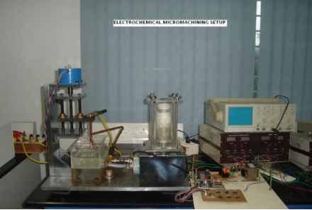
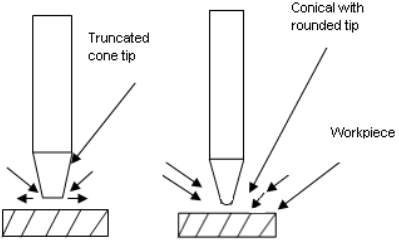
Figure 1 shows the developed EMM set-up. Essentially, the set-up incorporate different sub-systems and elements. The machining unit consists of the feeding attachment to the tool electrode, the main machining body, the machining chamber, and the work holding fixture. The body of the machine consists of MS and is plated with chromium for corrosion resistance. The 2 μm resolution tool electrode feed mechanism along the Z axis is designed with a stepper motor and an 8051 micro-controller. The experiments were conducted with a conical electrode diameter of 464 μm with rounded and truncated cone stainless steel, as shown in Figure 2.
Sodium nitrate (NaNO3) of different concentrations is used as an electrolyte, and low throwing power is preferred. The workpiece used was 304 stainless steel with a thickness of 200 μm. The tool is made as a cathode and workpiece is made as anode. L36 orthogonal array (OA) was chosen for experimentation for developing the ANN model. Experimental combination for L36 OA is shown in Table 1 [13-15].
Figure 1. EMM setup
Figure 2. Tool electrode tip shape
Table 1. Experimental combination for L36 orthogonal array
|
Tool Tip Shape |
Voltage (V) |
Puls On-Time (ms) |
Electrolyte Concentration (mole/l) |
Diameter (µm) |
OC (µm) |
Machining Time (sec) |
MR (µm/s) |
|
Conical with rounded |
8 |
7.5 |
20 |
472.5 |
11.25 |
57 |
3.51 |
|
Conical with rounded |
9 |
10 |
25 |
516.6 |
33.3 |
32 |
6.25 |
|
Conical with rounded |
10 |
15 |
30 |
627.9 |
88.95 |
17 |
11.76 |
|
Conical with rounded |
8 |
7.5 |
20 |
472.5 |
11.25 |
57 |
3.51 |
|
Conical with rounded |
9 |
10 |
25 |
516.6 |
33.3 |
32 |
6.25 |
|
Conical with rounded |
10 |
15 |
30 |
627.9 |
88.95 |
17 |
11.76 |
|
Conical with rounded |
8 |
7.5 |
25 |
506.7 |
28.35 |
52 |
3.85 |
|
Conical with rounded |
9 |
10 |
30 |
570.1 |
60.05 |
25 |
8 |
|
Conical with rounded |
10 |
15 |
20 |
556.3 |
53.15 |
23.5 |
8.51 |
|
Conical with rounded |
8 |
7.5 |
30 |
527.1 |
38.55 |
44 |
4.55 |
|
Conical with rounded |
9 |
10 |
20 |
516.6 |
33.05 |
41 |
4.88 |
|
Conical with rounded |
10 |
15 |
25 |
594.3 |
72.15 |
20 |
10 |
|
Conical with rounded |
8 |
10 |
30 |
546 |
48 |
28 |
7.14 |
|
Conical with rounded |
9 |
15 |
20 |
541.8 |
45.9 |
29 |
6.9 |
|
Conical with rounded |
10 |
7.5 |
25 |
502 |
26 |
29 |
6.9 |
|
Conical with rounded |
8 |
10 |
30 |
546 |
48 |
28 |
7.14 |
|
Conical with rounded |
9 |
15 |
20 |
541 |
45.9 |
29 |
6.9 |
|
Conical with rounded |
10 |
7.5 |
25 |
502 |
26 |
29 |
6.9 |
|
Truncated cone |
8 |
10 |
20 |
501.9 |
25.95 |
37 |
5.4 |
|
Truncated cone |
9 |
15 |
25 |
632.1 |
91.05 |
22 |
9.1 |
|
Truncated cone |
10 |
7.5 |
30 |
590.1 |
70.05 |
25 |
8 |
|
Truncated cone |
8 |
10 |
25 |
546 |
48 |
32 |
6.25 |
|
Truncated cone |
9 |
15 |
30 |
663.6 |
106.8 |
14 |
14.29 |
|
Truncated cone |
10 |
7.5 |
20 |
556.5 |
53.25 |
32 |
6.25 |
|
Truncated cone |
8 |
15 |
25 |
594.3 |
72.15 |
25 |
8 |
|
Truncated cone |
9 |
7.5 |
30 |
537.6 |
43.8 |
26 |
7.7 |
|
Truncated cone |
10 |
10 |
20 |
627.9 |
88.95 |
24 |
8.33 |
|
Truncated cone |
8 |
15 |
25 |
594.3 |
72.15 |
25 |
8 |
|
Truncated cone |
9 |
7.5 |
30 |
537.6 |
43.8 |
26 |
7.41 |
|
Truncated cone |
10 |
10 |
20 |
627.9 |
88.95 |
24 |
8.33 |
|
Truncated cone |
8 |
15 |
30 |
634.2 |
92.1 |
19 |
10.53 |
|
Truncated cone |
9 |
7.5 |
20 |
606.1 |
28.05 |
38 |
5.26 |
|
Truncated cone |
10 |
10 |
25 |
667.8 |
108.9 |
23 |
8.7 |
|
Truncated cone |
8 |
15 |
20 |
516.6 |
100.5 |
29 |
6.9 |
|
Truncated cone |
9 |
7.5 |
25 |
683 |
33.3 |
29 |
6.9 |
|
Truncated cone |
10 |
10 |
30 |
716.1 |
116.25 |
15 |
13.33 |
3.1 Configuration of ANN
The architecture of the network such as the number of layers and neurons are very significant factors that determine the network's generalization capacity and functionality. Standard multilayer feed forward neural networks employed with the MATLAB R2008 for this modeling.
Higher input variables that are valued may tend to resist the effect of shorter sizes. To solve this issues, the normalized neural networks were trained to learn the weights associated with the links emanating from these inputs, leaving it to the network. The input / output datasets were therefore normalized within the -1 and +1 range. For each raw output dataset / input dataset (yi), the normalized value (xi) was calculated based on Eq. (1).
$x_i=\frac{2\left(y_i-y_{\text {min }}\right)}{y_{\text {max }}-y_{\text {min }}}-1$ (1)
where, $\mathrm{y}_{\max }$ and $\mathrm{y}_{\min }$ are the maximum and minimum values of the raw data.
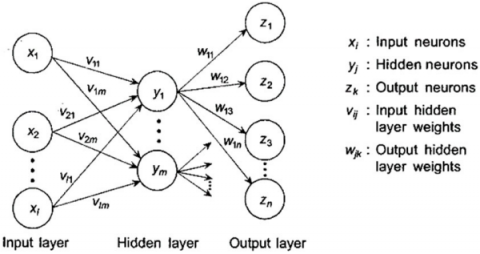
Networks consist of three or more layers: input, hidden layers, and layers of output. In Figure 3, the feed-forward ANN schema architecture developed with three inputs and four outputs is shown.
Figure 3. Feed-forward ANN schema architecture of developed with four outputs and three inputs
Different architectures have to be studied to determine the optimal architecture. The LMABR were used to train each network here. Due to its high accuracy in comparable function approximation, this training algorithm was chosen. In the output and hidden layer, the tangent sigmoid transfer function 'tansig' and linear transfer function 'purelin' have been used for all networks. The prediction error model in output node has been estimated as follows to test the ability of prediction.
$Prediction\,\, error\%=\frac{(\text { actual value-predicted value })}{\text { actual value }} \times 100$
The minimum, mean and maximum prediction errors for OC and MR were calculated and shown in Tables 2 and 3 for each network. For each model, the maximum percentage error specifies the worst prediction error. Table 4 shows the neural network performance with different OC and MR architectures.
Table 2. Performance of neural network with different architecture for OC
|
Network Architecture |
Maximum Prediction Error (%) |
Minimum Prediction Error (%) |
Mean Prediction Error (%) |
Correlation Coefficient |
|
4-15-2 |
1.431 |
-153.227 |
-58.867 |
0.873 |
|
4-20-2 |
46.988 |
-154.421 |
-18.005 |
0.403 |
|
4-25-2 |
56.027 |
-62.276 |
-4.882 |
0.763 |
|
4-30-2 |
60.027 |
-77.428 |
-2.111 |
0.605 |
|
4-32-2 |
46.781 |
-77.389 |
-27.6 |
0.931 |
|
4-35-2 |
1100.29 |
-105.431 |
119.502 |
0.801 |
|
4-2-2-2 |
49.251 |
-59.425 |
14.333 |
0.757 |
|
4-5-5-2 |
36.695 |
-163.022 |
-16.929 |
0.474 |
|
4-12-10-2 |
232.8676 |
-38.388 |
68.053 |
0.538 |
|
4-20-20-2 |
89.393 |
-159.204 |
-9.101 |
0.522 |
|
4-22-18-2 |
63.69 |
-733.059 |
-25.146 |
0.4 |
Table 3. Performance of neural network with different architecture for MR
|
Network Architecture |
Maximum Prediction Error (%) |
Minimum Prediction Error (%) |
Mean Prediction Error (%) |
Correlation Coefficient |
|
4-15-2 |
1.276 |
-43.1049 |
-4.719 |
0.637 |
|
4-20-2 |
56.816 |
-94.560 |
-10.442 |
0.647 |
|
4-25-2 |
37.520 |
-90.476 |
-21.635 |
0.505 |
|
4-30-2 |
158.518 |
-34.69 |
31.041 |
0.408 |
|
4-32-2 |
179.509 |
-32.771 |
34.710 |
0.905 |
|
4-35-2 |
149.54 |
-42.529 |
29.243 |
0.882 |
|
4-2-2-2 |
35.876 |
-32.179 |
0.956 |
0.769 |
|
4-5-5-2 |
31.032 |
-37.936 |
-1.153 |
0.731 |
|
4-12-10-2 |
139.57 |
-6.888 |
52.963 |
0.765 |
|
4-20-20-2 |
31.000 |
-50.771 |
-1.916 |
0.776 |
|
4-22-18-2 |
257.960 |
-65.548 |
26.6 |
0.757 |
Table 4. Neural network performance
|
Network Architecture |
Correlation Coefficient for Overcut |
Correlation Coefficient for Machining Rate |
|
4-15-2 |
0.873 |
0.637 |
|
4-20-2 |
0.403 |
0.647 |
|
4-25-2 |
0.763 |
0.505 |
|
4-30-2 |
0.605 |
0.408 |
|
4-32-2 |
0.931 |
0.905 |
|
4-35-2 |
0.801 |
0.882 |
|
4-2-2-2 |
0.757 |
0.769 |
|
4-5-5-2 |
0.474 |
0.731 |
|
4-12-10-2 |
0.538 |
0.765 |
|
4-20-20-2 |
0.522 |
0.776 |
|
4-22-18-2 |
0.4 |
0.757 |
The 4-32-2 architecture model is considered the most suitable. The rise in the number of neurons can be seen as from 30 to 32 in the hidden layer improves network performance and then decreases performance. Thus, the one hidden layer network consists of 32 neurons (4-32-2), trained with the LMABR, and was selected as the optimum network and used to model the OC and MR.
This paper introduces a method using the LevenbergMarquardt algorithm to optimize EMM process parameters. To represent the relation between MR, OC and input parameters, an ANN model was developed. The model with the 4-32-2 architecture is the most suitable. The rise in the number of neurons can be seen as from 30 to 32 in the hidden layer improves network performance and then decreases performance. Therefore, 32 neurons (4-32-2), trained with the LMABR, consist of a network with one hidden layer and were chosen as the optimum network and used to model the OC and MR. This demonstrates that the net has better generalization efficiency, and the speed of convergence is faster.
[1] Yi. Qin, A. Brockett, Y. Ma, A. Razali, J.Zhao, C.Harrison, W.Pan X.Dai & D.Loziak, “Micromanufacturing: research, technology outcomes and development issues”, Intl Journal of Adv Mfg Tech, vol.47, 2010, pp 821–837.
[2] B.Bhattacharyya, J.Munda, & M.Malapati, “Advancement in electrochemical micromachining”, (2004). J Mach Tools Manuf, Vol.44, 2004, pp1577-1589.
[3] K.M. Tsai, P.J.Wang, “Predictions on surface finish in electrical discharge machining based upon neural network models”, International Journal of Machine Tools and Manufacture, Vol.41, 2001,pp. 1385-1403.
[4] F.G.Cao, Yang, D.Y. “The study of high efficiency and intelligent optimization system in EDM sinking process”, Journal of Materials Processing Technology, Vol.149 (1- 3): 2004, pp.83-87.
[5] Qing GAO, Qin-he ZHANG, Shu-peng SU, Jian-hua ZHANG “Parameter optimization model in electrical discharge machining process”, J Zhejiang Univ Sci A Vol. 9(1):2008,pp.104-108
[6] Catalin Sorin UNGUREANU, “Modelling And Simulation of The Electrochemical Machining Using Neural Networks”, http://www.fs.vsb.cz/transactions/2006- 2/1557_ungurenu_catalin_sorin.pdf, pp 197-202.
[7] Kumar, K. S., & Sivasubramanian, R. (2011). Modeling of metal removal rate in machining of aluminum matrix composite using artificial neural network. Journal of composite materials, 45(22), 2309-2316.
[8] Sangwan, K. S., Saxena, S., & Kant, G. (2015). Optimization of machining parameters to minimize surface roughness using integrated ANN-GA approach. Procedia CIRP, 29, 305-310.
[9] Zou, P., Rajora, M., Ma, M., Chen, H., Wu, W., & Liang, S. Y. (2017, January). Electrochemical Micro-Machining Process Parameter Optimization Using a Neural NetworkGenetic Algorithm Based Approach. In Proceedings of the International Conference on Manufacturing Technologies, San Diego, CA, USA (pp. 19-21).
[10] Kasdekar, D. K., Parashar, V., & Arya, C. (2018). Artificial neural network models for the prediction of MRR in Electro-chemical machining. Materials Today: Proceedings, 5(1), 772-779.
[11] Maniraj, S., & Thanigaivelan, R. (2019). Optimization of Electrochemical Micromachining Process Parameters for Machining of AMCs with Different% Compositions of GGBS Using Taguchi and TOPSIS Methods. Transactions of the Indian Institute of Metals, 72(12), 3057-3066.
[12] Kalaimathi, M., Venkatachalam, G., & Sivakumar, M. (2020). An experimental investigation and modelling for travelling wire electrochemical machining of Monel 400 alloys. International Journal of Manufacturing Technology and Management, 34(3), 259-281.
[13] Viswanathan, R., Ramesh, S., Maniraj, S., & Subburam, V. (2020). Measurement and Multi-response Optimization of Turning Parameters for Magnesium Alloy Using Hybrid Combination of Taguchi-GRA-PCA Technique. Measurement, 107800.
[14] Babu, B., Sabarinathan, C., Dharmalingam, S., (2020). Production of Aluminum 6063 Metal Matrix Composite with 12% Magnesium Oxide and 5% Graphite and its Machinability Studies using Micro Electrochemical Machining, Journal of New Materials for Electrochemical Systems.23, 94-100. https://doi.org/10.14447/jnmes.v23i2.a06.
[15] Rajan, N., Thanigaivelan, R., Muthurajan, K.G., (2018). Effenct of Electrochemical Machining Process Parameters on Anisotropic Property of Metal Matrix Composites Al7075, Journal of New Materials for Electrochemical Systems.21, 239-242. https://doi.org/10.14447/jnmes.v21i4.a08
[16] Pravin Pawar., Amaresh Kumar., Raj Ballav., (2020). Grey Relational Analysis Optimization of Input Parameters for Electrochemical Discharge Drilling of Silicon Carbide by Gunmetal Tool Electrode. Annales de Chimie - Science des Matéria 44, 239 – 249. https://doi.org/10.18280/acsm.440402.