Ahmed F. Mutlak*![]() | Amjad Jaleel Humaidi
| Amjad Jaleel Humaidi![]()
© 2023 IIETA. This article is published by IIETA and is licensed under the CC BY 4.0 license (http://creativecommons.org/licenses/by/4.0/).
OPEN ACCESS
This study presents a performance comparison between a synergetic controller (SC) and a sliding mode controller (SMC) applied to a pendulum System. Initially, the mathematical model of the pendulum system is established. Subsequently, the design of both synergetic and sliding mode controls is elaborated, leading to the development of control laws for the proposed controllers. The effectiveness of the pendulum system controlled by SC and SMC has been validated through numerical simulations. These simulations revealed that the control signal exhibits chattering behaviour in the case of SMC, while this phenomenon is absent with the SC, demonstrating a distinct difference in performance between the two control systems.
synergetic control, sliding mode control, pendulum system, chattering phenomenon, control design
Most nonlinear systems have uncertain dynamic properties. As a result, controllers that are both high-performance and robust are needed. Recently, advanced algorithms have been used to design nonlinear controllers that are resilient and provide the required performance. One of them is the synergetic controller (SC) and sliding mode controller. It is a nonlinear and robust controller that may be used specifically with nonlinear systems whose parameters are uncertain. The sliding mode control (SMC) has been designed to ensure finite-time convergence of the sliding mode system dynamics. The sliding mode control utilizes nonlinear sliding surfaces instead of linear planes. SMC provides the benefit of finite time convergence and little steady-state error [1]. However traditional sliding mode control has singular points. The singularity can be avoided with non-singular sliding mode control, but the upper bounds of the disturbances must typically be known in order to calculate the switching gain [2, 3]. Synergetic control, which is similar to sliding mode control, is predicated on the idea that by using a continuous control law to guide a system to a wanted manifold with designer-selected dynamics, we can achieve results that are competitive with SMC while avoiding the latter's main drawback, chattering. The SC has the advantages of finite time convergence and low steady-state error. This control is crucial to the reliable operation of the pendulum system [4]. Recent control techniques and applied control to pendulum systems are discussed in the following literature: Tohma and Hamoudi [5] produced A study comparing the ASMC with the CSMC for simple pendulum found that the former was better at minimizing control action and chattering by setting the controller gain to an optimally small amount. Yakubu, Olejnik and Awrejcewic [4] proved the systemic impact of a variable pendulum length. The system's vertically stimulated parametric pendulum with variable length is constructed, resulting in quicker and longer oscillations than those of the constant-length pendulum. Hence, greater and more complex dynamics are realized. Ali and Naji [6] presented are designs for state feedback and state feedback with integrated controllers for the rotary inverted pendulum system. Using PSO, they were able to determine the ideal values for the state feedback gains. The suggested cost function incorporates the time response standards and restrictions to ensure that it is both resilient and able to fulfil the time response demands. To further track the system, state feedback plus integral was developed. Humaidi et al. [7] introduced an adaptive observer-based nonlinear backstepping control architecture. Both the reduced order adaptive observer and the backstepping design aim to predict the velocities of the cart and the pole, respectively. By means of simulated data in the MATLAB, the efficacy of an observer-based backstepping controller has been tested. Mokhtari et al. [8] developed adaptive neural network based on backstepping approach to a simple pendulum with in face of model uncertainties and perturbations. Berrahal et al. [9] developed observer-based adaptive backstepping that use the simple pendulum as an illustration. Using the observer technique, the adaptive backstepping control is examined.
In this study, two control design has been developed to control the angular position of simple inverted pendulum system. The first control approached is developed based on synergetic control theory, while the second control approach is established based on sliding mode control methodology.
The Contribution of this Work can be summarized:
A free body diagram of the system is shown in Figure 1 [10]. It is instructive to work out this equation of motion also using Lagrangian mechanics. The Lagrangian function is defined as
$L=T-U$ (1)
where, T is the total kinetic energy and U is the total potential energy of the mechanical system.
Figure 1. Free body of simple pendulum
To get the equations of motion, we use the Lagrangian formulation
$\frac{d}{d t}\left(\frac{\partial L}{\partial \dot{q}_i}\right)-\left(\frac{\partial L}{\partial q_i}\right)=F_i$ (2)
where, q signifies generalized coordinates and F signifies non-conservative forces acting on the mechanical system. For the simplify pendulum, we assume no friction, so no non-conservative forces, so all Fi are 0. The aforementioned equation of motion is in terms of $\theta_p$ as a coordinate, not in terms of x and y. So we need to use kinematics to get our energy terms in terms of $\theta_p$.
The linear velocity of the mass vm is given by:
$v_m=l . \dot{\theta}_p$ (3)
The total kinetic energy T can be described by:
$T=\frac{1}{2} m v_m^2$ (4)
Using Eq. (3), Eq. (4) can be rewritten as:
$T=\frac{1}{2} m l^2 \dot{\theta}_p^2$ (5)
The potential energy, U, depends only on the y-coordinate. Taking $\theta_p=0$ as the position where U=0,
$y=l-l \cos \theta_p$ (6)
Then, the potential energy U is given by:
$U=m . g . y=m . g . l .\left(1-\cos \theta_p\right)$ (7)
Now we have all the parts and pieces to complete the Lagran gian formulation. The Lagrangian function in terms of $\theta_p$ is
$L=T-U=\frac{1}{2} m l^2 \dot{\theta}_p^2-m . g . l .\left(1-\cos \theta_p\right)$ (8)
Using $q_1=\theta_p$ , the elements of Eq. (2) can be given by:
$\frac{\partial L}{\partial \dot{\theta}_p}=m \cdot l^2 \cdot \dot{\theta}_p$ (9)
$\frac{d}{d t}\left(\frac{\partial L}{\partial \dot{\theta}_p}\right)=m . l^2 . \ddot{\theta}_p$ (10)
$\frac{\partial L}{\partial \theta_p}=-m . g . l . \sin \theta_p$ (11)
Now, putting these last two equations together
$\frac{d}{d t}\left(\frac{\partial L}{\partial \dot{\theta}_p}\right)-\frac{\partial L}{\partial \theta_p}=m . l^2 . \ddot{\theta}_p+ m.g.l. \sin \theta_p=\tau_p$ (12)
Let $x_1=\theta$ and $x_2=\dot{\theta}_p$, and $u=\tau_p$, the equation of state variables
$\dot{x}_1=x_2$ (13)
$\dot{x}_2=-\frac{g}{l} \sin \left(x_1\right)+\frac{1}{m l^2} u$ (14)
where, l is the length of the pendulum in meters, g is the acceleration due to gravity, m is mass of the pendulum and u control action ($\tau$ torque of pendulum). For simplicity, Eq. (14) can be written in the following form:
$\dot{x}_2=f+b u$ (15)
where, $f=-g \sin \left(x_1\right) / l, b=1 /\left(m L^2\right)$.
3.1 Control design based on synergetic control
Let $\epsilon$ the error between the actual angle position $x_1=\theta$ and the desired $x_{1d}=\theta_d$ as follows:
$\epsilon=x_1-x_{1 d}$ (16)
Taking the first and second derivatives, one can have
$\dot{\epsilon}=\dot{x}_1-x_{1 d}^{\cdot}=x_2-x_{1 d}^{\cdot}$ (17)
$\ddot{\epsilon}=\dot{x}_2-\ddot{x}_{1 d}=f+b u-\ddot{x}_{1 d}$ (18)
Let $\varphi(\epsilon)$ be defined as:
$\varphi(\epsilon)=\alpha \epsilon+\dot{\epsilon}$ (19)
Taking the derivative of Eq. (19), one can obtain
$\dot{\varphi}(\epsilon)=\dot{\epsilon}+\alpha \ddot{\epsilon}$ (20)
where, $\alpha$ is a scalar design for synergetic control. The definition of the $\varphi(\epsilon)$ with respect to the manifolds is given by
$T \dot{\varphi}(\epsilon)+\varphi(\epsilon)=0$ (21)
where, T>0 is responsible for converging ratio of $\varphi(\epsilon)$ to manifold $\varphi(\epsilon)=0$.
Using Eq. (20), Eq. (21) becomes
$T(\dot{\epsilon}+\alpha \ddot{\epsilon})+\varphi(\epsilon)=0$ (22)
$T \dot{\epsilon}+T \alpha \ddot{\epsilon}+\varphi(\epsilon)=0$ (23)
Using Eq. (17) and Eq. (18)
$T \dot{\epsilon}+T \alpha f+T \alpha b u-T \alpha \ddot{x}_{1 d}+\varphi(\epsilon)=0$ (24)
According to Eq. (24), the control law can be deduced
$u_{s c}=\frac{1}{T \alpha b}\left(-T \dot{\epsilon}-T \alpha f-\varphi(\epsilon)+T \alpha \ddot{x}_{1 d}\right)$ (25)
where, $u_{s c}$ represents the control action to pendulum system based on synergetic control.
3.2 Control design slide mode controller
In sliding mode control, the control law consists of two parts: equivalent part and switching part. The equivalent part of control signal is responsible for bringing the trajectory from initial states to the sliding surface, while the switching part tries to keep the trajectory on the sliding surface until reaches the origin [11, 12]. The sliding surface is given by
$s=c \epsilon+\dot{\epsilon}$ (26)
where, c is scalar design parameter of positive value. The time derivative of Eq. (26) is given by
$\dot{s}=c \dot{\epsilon}+\ddot{\epsilon}$ (27)
Using Eq. (18) to have
$\dot{s}=c \dot{\epsilon}+f+b u_n-\ddot{x}_{1 d}$ (28)
Setting $\dot{s}=0$, the equivalent control law can be deduced
$u_n=\frac{1}{b}\left(-c \dot{\epsilon}+f+\ddot{x}_{1 d}\right)$ (29)
$u_n=m L^2\left(-c \dot{\epsilon}+\frac{g}{L} \sin \left(x_1\right)+\ddot{x}_{1 d}\right)$ (30)
The total control law can be composed by adding the equivalent control part to switching part
$u=u_n+u_s$ (31)
where, $u_n$ represents the nominal (equivalent) control and $u_s$ denotes the discontinuous control part, which is defined by
$u_s=-\kappa\,\, {sign}(s)$ (32)
where, $\kappa$ is a gain of positive value. As a result, the formula of control law can be given by
$u_{s m c}=m L^2\left(-c \dot{\epsilon}+\frac{g}{L} \sin \left(x_1\right)+\ddot{x}_{1 d}\right)-\kappa {sign}(s)$ (33)
According to above analysis, two important remarks can be deduced [13, 14]:
Remarks 1: The control signal in synergetic control is continuous without interruptions, while there is chattering behavior.
Remark 2: According to Eq. (21), the synergetic control enforces the dynamic characteristics towards the manifold $(\epsilon)=0$. The time constant T in Eq. (21) permits the change of the convergence rate of trajectory towards $\varphi(\epsilon)=0$.
The effective of controllers have been verified via numerical simulation. The Simulink blocks within MATLAB environment has been used to represent the dynamic model of pendulum system and to synthesize synergetic and sliding mode controllers using Matlab functions. The codes used in developing the control algorithms reside inside these M-functions which are present within the library of MATLAB/Simulink. The block diagram of Figures 2 and 3 has been modelled by Simulink blocks for both controlled pendulum systems based on synergetic and slide mode controllers.
Figure 2. The schematic diagram of synergetic controlled pendulum system
Figure 3. The schematic diagram of sliding mode controller for pendulum system
The parameters of pendulum system is selected as follows [8]:
$m=0.23 \mathrm{~kg}, L=0.5 m$, and $g=9.81 \mathrm{~m} / \mathrm{s}^2 \mathrm{~m}$
The selected parameters of the synergetic and slide mode controller are as follows [7]:
$T=0.1, \alpha=2.3, c=2.3$ and $\kappa=2.4$
The external disturbance value $\delta_1=0.2$ and $\delta_2=0.3$.
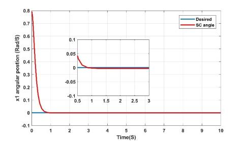
Both SC and SMC controllers have been applied to control the angular positions of pendulum system. Figures 4 and 5 show the behaviour of angular position under the control of proposed controllers. Figures 6 and 7 show the responses of tracking errors based on SC and SMC, respectively. It is clear that the controllers shows the can asymptotic stability of controlled system.
Synergetic control and sliding mode control are both used to control the angular velocity of a simple pendulum. The first and second controllers depicted in Figures 8 and 9 are extremely close to providing the pendulum's angular velocity.
Figure 4. Tracking performance pendulum system using synergetic controller
Figure 5. Tracking performance for pendulum system using sliding mode control
Figure 6. Tracking error for synergetic controller
Figure 7. Tracking error for synergetic controller
Figure 8. Angular velocity for simple pendulum using synergetic controller
Figure 9. Angular velocity for simple pendulum using sliding mode controller
Figures 10 and 11 represent control action of pendulum, When the signum function is applied to the controller law, it causes the chattering phenomenon that affects SMC. In contrast, with SC controller, the control signal is modified, and there is no chattering phenomenon without the use of any chattering treatment tools.
To evaluate the system's robustness, the mass of the pendulum (m) and the length of the pendulum (L) are adjusted by 25%. Figures 12 and 13 depict the system response when the parameters are uncertain. It is demonstrated that the system is stable in spite of changes in system parameters. This indicates that proposed tow controllers may successfully compensate for system parameter changes.
Figure 10. Control action for synergetic controller
Figure 11. Control action for sliding mode controller
Figure 12. Uncertain system response using synergetic controller
Figure 13. Uncertain system response using sliding mode controller
Table 1 shows the Performance between the SC and SMC controlled Pendulum systems. In a numerical sense, the RMSE value resulting from SC is equal to 0.1235 rad, while the RMSE given by SM is equal to 0.2756 rad. This indicates that the SC gives better performance and better error variance. This means that the synergetic controller gives greater resistance to changing parameters than the sliding mode controller, and therefore the SC controller is more Robust than the SMC controller.
Table 1. Performance between the SC and SMC controlled pendulum systems
|
Controller |
Nominal Parameter (m, L) |
% Variation |
Uncertain Parameter (m, L) |
ERMS |
|
SC |
0.25 |
25% |
0.3125 |
0.1235 |
|
SMC |
0.5 |
25% |
0.625 |
0.2756 |
Figure 14. Angular response using synergetic controller under external disturbance
Figure 15. Angular response using sliding mode control under external disturbance
In the next scenario, the robustness characteristics of both controller have been evaluated by injecting disturbances on both channels of pendulum system. Actually, the basic pendulum dynamic equations, described by Eq. (3) and Eq. (4), can be rewritten as
$\dot{x}_1=x_2+\delta_1$ (34)
$\dot{x}_2=-\frac{g}{L} \sin \left(x_1\right)+\frac{1}{m L^2} u+\delta_2$ (35)
where, $\delta_1$ and $\delta_2$ represents the external disturbance added to the system. Figures 14 and 15 show the effect of the external disturbance on the transient response of controlled system based on SC and SMC, respectively. The robustness of controllers are assessed by evaluating the deviation between the nominal response and the deviated response due to load application. The Root Mean Square of t Deviation (RMSD) has been calculated for both controllers. It turns out that the SC gives less RMSD (0.2634) than that based on SMC (0.2785). This leads to conclusion that the SC is more robust than SMC.
As future extension of this study, other control schemes can be used to control the pendulum system [15-20], or one can use modern optimization techniques to tune the design parameters of SC and SMC towards their improvement [21-25].
In this paper, the design and simulation of two controllers has been present for simple pendulum system. The first control design is based on synergetic theory and the second control design is based on SMC. The MATLAB programming software is used to simulate and verify the effectiveness of both controllers. The simulated results showed that the SC has better transient and robustness characteristics as compared to SMC. Moreover, the SC has no chattering behavior as compared to high chattering effect resulting from the SMC.
|
L |
Length of the pendulum m |
|
m |
Mass The of the pendulum kg |
|
g |
Acceleration due to gravity |
|
$\tau$ |
Torque of pendulum N.m |
|
$\epsilon$ |
The error between the actual angle position and the desired |
|
T |
The converging ratio of $\varphi(\epsilon)$ to manifold |
|
u |
Control action N.m |
|
c |
A scalar design for sliding mode control |
|
$u_{sc}$ |
Control action of synergetic control |
|
$u_{n}$ |
Nominal slide mode controller |
|
$u_{dis}$ |
Discontinuous control action (sliding mode control) |
|
s |
Sild surface of slide mode control |
|
$\kappa$ |
Gain design for sliding mode control (Discontinues) |
|
Greek symbols |
|
|
$\theta$ |
Angular position |
|
$\dot\theta$ |
Angular velocity |
|
$\ddot\theta$ |
Angular acceleration |
|
$\theta_d$ |
Desired angle Rad |
|
$\alpha$ |
A scalar design for synergetic control |
|
$\varphi(\epsilon)$ |
Manifold of synergetic control |
|
$\delta_1$ |
External disturbance 1 |
|
$\delta_2$ |
External disturbance 2 |
|
Subscripts |
|
|
SC |
Synergetic control |
|
SMC |
Sliding mode control |
|
RMSE |
Root mean square error |
[1] Komurcugil, H. (2012). Adaptive terminal sliding-mode control strategy for DC–DC buck converters. ISA Transactions, 51(6): 673-681. https://doi.org/10.1016/j.isatra.2012.07.005
[2] Neila, M.B.R., Tarak, D. (2011). Adaptive terminal sliding mode control for rigid robotic manipulators. International Journal of Automation and Computing, 8: 215-220. https://doi.org/10.1007/s11633-011-0576-2
[3] Teja, S.V., Shanavas, T.N., Patnaik, S.K. (2012). Modified PSO based sliding-mode controller parameters for buck converter. In 2012 IEEE Students' Conference on Electrical, Electronics and Computer Science, Bhopal, India, pp. 1-4. https://doi.org/10.1109/SCEECS.2012.6184759
[4] Yakubu, G., Olejnik, P., Awrejcewicz, J. (2021). Modeling, simulation, and analysis of a variable-length pendulum water pump. Energies, 14(23): 8064. https://doi.org/10.3390/en14238064
[5] Tohma, D.H., Hamoudi, A.K. (2021). Design of adaptive sliding mode controller for uncertain pendulum system. Engineering and Technology Journal, 39(3): 355-369. https://doi.org/10.30684/etj.v39i3A.1546
[6] Ali, H.I., Naji, R.M. (2016). Optimal and robust tuning of state feedback controller for rotary inverted pendulum. Engineering and Technology Journal, 34(15): 2924-2939. https://doi.org/10.30684/etj.34.15A.13
[7] Humaidi, A.J., Tala'at, E.N., Hameed, M.R., Hameed, A.H. (2019). Design of adaptive observer-based backstepping control of cart-pole pendulum system. In 2019 IEEE International Conference on Electrical, Computer and Communication Technologies (ICECCT), Coimbatore, India, pp. 1-5. https://doi.org/10.1109/ICECCT.2019.8869179
[8] Mokhtari, M., Chara, K., Golea, N. (2014). Adaptive neural network control for a simple pendulum using backstepping with uncertainties. International Journal of Advanced Science and Technology, 65: 81-94. http://dx.doi.org/10.14257/ijast.2014.65.07
[9] Mokhtari, M., Golea, N., Berrahal, S. (2008). The observer adaptive backstepping control for a simple pendulum. AIP Conference Proceedings, 1019(1): 85-90. https://doi.org/10.1063/1.2953059
[10] Robinett, R.D., Dohrmann, C.R., Eisler, G.R., Feddema, J.T., Parker, G.G., Wilson, D.G., Stokes, D. (2002). Nonlinear systems and sliding mode control. In: Flexible Robot Dynamics and Controls. International Federation for Systems Research International Series on Systems Science and Engineering, vol 19. Springer, Boston, MA. https://doi.org/10.1007/978-1-4615-0539-6_7
[11] Husain, S.S., Ridha T.M. (2022). Design of integral sliding mode control for seismic effect regulation on buildings with unmatched disturbance. Mathematical Modelling of Engineering Problems, 9(4): 1123-1130. https://doi.org/10.18280/mmep.090431
[12] Humaidi, A.J., Hameed, A.H. (2018). PMLSM position control based on continuous projection adaptive sliding mode controller, Systems Science & Control Engineering, 6(3): 242-252. https://doi.org/10.1080/21642583.2018.1547887
[13] Abderrezek, H., Harmas, M.N. (2015). Comparison study between the terminal sliding mode control and the terminal synergetic control using PSO for DC-DC converter. In 2015 4th International Conference on Electrical Engineering (ICEE), Boumerdes, Algeria, pp. 1-5. https://doi.org/10.1109/INTEE.2015.7416609
[14] Al-Dujaili, A.Q., Humaidi, A.J., Allawi, Z.T., Sadiq, M.E. (2023). Earthquake hazard mitigation for uncertain building systems based on adaptive synergetic control. Applied System Innovation, 6(2): 34. https://doi.org/10.3390/asi6020034
[15] Kasim, M.Q. Hassan, R.F. (2021). Reduced computational burden model predictive current control of asymmetric stacked multi-level inverter based STATCOM. 2021 IEEE International Conference on Automatic Control & Intelligent Systems (I2CACIS), Shah Alam, Malaysia, pp. 374-379.
[16] Noaman, N.M., Gatea, A.S., Humaidi, A.J., Kadhim, S.K., Hasan, A.F. (2023). Optimal tuning of PID-controlled magnetic bearing system for tracking control of pump impeller in artificial heart. Journal Européen des Systèmes Automatisés, 56(1): 21-27. https://doi.org/10.18280/jesa.560103
[17] Husain, S.S., Ridha T.M. (2022). Integral sliding mode control for seismic effect regulation on buildings using ATMD and MRD. Journal Européen des Systèmes Automatisés, 55(4): 541-548. https://doi.org/10.18280/jesa.550414
[18] Al-Azzawi, R.S., Simaan, M.A. (2018). Sampled closed-loop control in multi-controller multi-objective control systems. In SoutheastCon 2018, St. Petersburg, FL, USA, pp. 1-7. https://doi.org/10.1109/SECON.2018.8478971
[19] Nasser, T.H., Hamza, E.K., Hasan, A.M. (2023). MOCAB/HEFT algorithm of multi radio wireless communication improved achievement assessment. Bulletin of Electrical Engineering and Informatics, 12(1): pp. 224–231. https://doi.org/10.11591/eei.v12i1.4078
[20] Mohammed, A.M., Al-Samarraie, S.A., Jaber, A.A. (2022). Design of a robust controller for a gearbox connected two-mass system based on a hybrid model. FME transactions, 50(1): 79-89. https://doi.org/10.5937/fme2201079M.
[21] Dhomad, T.A., Jaber, A.A. (2020). Bearing fault diagnosis using motor current signature analysis and the artificial neural network. International Journal on Advanced Science, Engineering and Information Technology, 10(1): 70-79. https://doi.org/10.18517/ijaseit.10.1.10629
[22] Waheed, Z.A., Humaidi, A.J. (2022). Design of optimal sliding mode control of elbow wearable exoskeleton system based on whale optimization algorithm. Journal Européen des Systèmes Automatisés, 55(4): 459-466. https://doi.org/10.18280/jesa.550404.
[23] Humaidi, A.J., Hameed, A.H., Hameed, M.R. (2017). Robust adaptive speed control for DC motor using novel weighted E-modified MRAC. In 2017 IEEE International Conference on Power, Control, Signals and Instrumentation Engineering (ICPCSI), Chennai, India, pp. 313-319. https://doi.org/10.1109/ICPCSI.2017.8392302.
[24] Al-Azzawi, R.S., Simaan, M.A. (2019). Leader-follower controls in systems with two controllers. In 2019 SoutheastCon, Huntsville, AL, USA, pp. 1-6. https://doi.org/10.1109/SoutheastCon42311.2019.9020435
[25] Al-Azzawi, R.S., Simaan, M.A. (2021). On the selection of leader in Stackelberg games with parameter uncertainty. International Journal of Systems Science, 52(1): 86-94. https://doi.org/10.1080/00207721.2020.1820097