Nacereddine Djelal*![]() | Abdelhak Ouanane
| Abdelhak Ouanane![]() | Fares Bouriachi
| Fares Bouriachi![]()
© 2023 IIETA. This article is published by IIETA and is licensed under the CC BY 4.0 license (http://creativecommons.org/licenses/by/4.0/).
OPEN ACCESS
This paper introduces a novel application of the Long Short-Term Memory (LSTM) recurrent neural network for the identification and control of complex systems. The computation-intensive task of calculating the interaction matrix, a necessity for visual control laws in these systems, makes LSTM a fitting solution. The proposed control law unfolds in two phases: an offline phase, where the LSTM is trained on a set of visual features to generate a kinematic screw vector, and an online phase, where the trained LSTM is utilized for real-time system control. To assess the efficacy of the LSTM-based approach, we undertook a case study involving a manipulator robot, the UR5. We executed a series of simulations under various conditions to illustrate the effectiveness of the proposed LSTM-based control law. The outcomes from these experiments affirm the robustness of the LSTM controller, outperforming traditional methods even when faced with rapid fluctuations in visual features, partial loss of visual information, and model uncertainties in the robot.
visual servoing, interaction matrix, 6DOF robot, LSTM, identification
Intelligent robots can interact safely with their environment and perform tasks that resemble human actions, thanks to the utilization of exteroceptive sensors such as cameras. Cameras provide abundant information about the environment, and algorithms extract visual features that can be used to synthesize a vision control law. In recent years, researchers have addressed the problems in visual servoing [1]. Most of these control laws are based on regulating a task function that minimizes the error between the actual and measured visual data. The traditional approach involves calculating the interaction matrix (visual Jacobian) and its pseudo-inverse for each visual feature point. However, these conventional controllers have large interaction matrices and pseudo-inverses, which significantly increase calculation time, particularly for complex visual trajectories. Additionally, conventional controllers are unable to compensate for lost visual information.
Visual control is inherently challenging due to the complex and ever-changing nature of visual data in real-world settings. Images and video frames contain a lot of information, and environmental conditions, object positions, and scene configurations can vary unpredictably. Traditional control methods often struggle to adapt to this complexity and variability. LSTM, a type of neural network, is a favored solution for visual control due to its unique attributes. LSTMs excel at handling non-linear relationships between visual input and control actions, capturing temporal dependencies in data, and adapting to different tasks through training. They are well-suited for real-time processing, making them valuable in dynamic environments.
Furthermore, LSTMs have a well-established history of success in various domains, prompting their exploration in visual control applications where complex, high-dimensional, and dynamic visual data requires effective management.
Shi et al. [2] proposed a fuzzy adaptive method for decoupled image-based visual servoing (IBVS) to enhance the performance of a mobile robot's control. This method enables efficient control by addressing the under-actuated dynamics through the decoupling of translation and rotation, achieved by using two independent servoing gains, as opposed to the single servoing gain used in traditional IBVS. To improve convergence, the study incorporates an improved Q-learning approach to adaptively adjust the parameters of the image Jacobian matrix. Furthermore, the fuzzy method is utilized to tune the learning rate of the Q-learning technique.
Wang [3] have introduced innovative techniques for vision-based robotic manipulation tasks, specifically visual servoing. These tasks involve positioning the object at specific angles or shapes for further operations. The authors proposed a method that incorporates Bezier curves and non-uniform rational b-spline (NURBS) curves to accurately fit the object's contour and extract its image contour features. These features are then utilized to provide visual feedback on the object's shape to the eye-in-hand visual servoing system. By using this visual feedback, the system controls the robot's movements and guides it to converge the image features to the desired values, allowing precise positioning of the object for subsequent operations. Notably, their proposed method does not rely on prior knowledge of the object's 3D position, as it employs adaptive laws to estimate curve parameters online.
In examining the limitations of various existing methods, we find that feedforward neural networks (FNNs) are designed primarily for static data processing, lacking inherent temporal awareness needed for tasks involving time-series data or dynamic visual control. Their training demands intricate model tuning with a multitude of hyperparameters, potentially time-consuming and requiring expertise. Furthermore, FNNs often require a huge amount of labeled data, presenting challenges in scenarios where obtaining such data is costly or challenging. Fuzzy logic, another approach, relies on manually defined rules and membership functions, posing difficulties in crafting accurate rules for complex systems. It also lacks the autonomous learning capabilities essential for dynamic environments. While renowned for interpretability, achieving high performance in fuzzy logic often entails complex rule sets, compromising the system's interpretability-performance balance. Hybrid systems that merge fuzzy logic and neural networks encounter challenges in integrating these components seamlessly, potentially diminishing interpretability and straightforward learning. Additionally, generating effective fuzzy rules from data remains a complex task, and suboptimal rules may adversely affect system performance. It's essential to recognize that these limitations vary with context, and these methods, while constrained, continue to have value, often complementing other techniques in response to specific problem requirements and constraints. The LSMT method overcomes the limitations of the FFNs and fuzzy logic.
The Long Short-Term Memory is a specific type of neural network architecture designed to model complex sequences and patterns using a recursive structure. Unlike other neural networks, the LSTM can retain information over extended periods, making it adept at learning and predicting complex temporal relationships. In the literature, the most commonly used variant of the LSTM is known as the vanilla LSTM, which was initially proposed by Graves and Schmidhuber. This variant typically comprises a single memory unit and only one recursive connection, a configuration that has proven to be effective for a wide range of sequence modeling tasks. Examples of such tasks include speech recognition, natural language processing, and image captioning [4-6].
Despite its success, the vanilla LSTM model has limitations in terms of its ability to capture long-term dependencies and handle noisy data. To address these issues, researchers have developed a variety of modified LSTM architectures, such as the peephole LSTM, the gated recurrent unit (GRU) and the attention-based LSTM. These variants have been shown to outperform the vanilla LSTM on certain tasks and are widely used in both academic research and industry applications.
Liu et al. [7] utilized deep neural networks (DNNs) and LSTM to develop models for robot inverse dynamics, demonstrating the application of deep learning techniques. Rueckert et al. [8] also presented an inverse dynamics prediction model for manipulators based on LSTM, and their model exhibited satisfactory predictive performance. This increasing trend in using deep learning techniques for developing robot inverse dynamics models emphasizes the growing importance of artificial intelligence in robotics research and development.
Motivated by the previously proposed techniques, in this paper, we introduce a new approach, leveraging LSTM for adept control and optimization in complex systems with refined precision and adaptability. It not only inherits the robust memory and learning capabilities of LSTM in system control, producing a methodology that is both innovative and practically astute. Subsequent sections will delve into a detailed discourse on the various advantages brought forth by our LSTM-based approach, exploring its potential and applicability in control of robotics systems, which can offer several advantages that can be outlined as follows:
The outline of the paper is as follows: We start by modeling a six DOF arm robot. Next, an overview of the conventional vision control law will be provided, and an enhanced robust visual controller will be suggested. Finally, the results obtained from the implementation of the proposed robust vision control law will be evaluated and discussed.
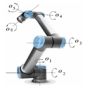
This section focuses on the use of the well-known UR5 robot [9, 10] to validate the control law, which is illustrated in Figure 1. The robot has 6 degrees of freedom and the camera is attached to its end-effector. The forward geometric model of the robot [11] is calculated by using Craig notation [12-14]. The transformations between the two successive links are calculated by using the Denavit-Hartenberg notation (Table 1). In addition, the UR5 robot produced by Universal Robots is also depicted on Figure 1.
Figure 1. Kinematic parameters and frame assignments of the UR5
Table 1. Denavit-Hartenberg parameters of the UR5
|
Link |
$a_i$ |
$a_i$ |
$d_i$ |
$\boldsymbol{\theta}_i$ |
|
1 |
0 |
90° |
0.0891 |
$\theta_1$ |
|
2 |
-0.425 |
0° |
0 |
$\theta_2$ |
|
3 |
-0.392 |
0° |
0 |
$\theta_3$ |
|
4 |
0 |
90° |
0.109 |
$\theta_4$ |
|
5 |
0 |
-90° |
0.0946 |
$\theta_5$ |
|
6 |
0 |
0° |
0.0823 |
$\theta_6$ |
The UR5 is characterized by 6 degrees of freedom [9, 10]. It can work safely alongside employees or separately and can carry loads up to 10kg. Its reach radius is 1300mm with a rotation of 360° for each joint. Its weight is 33.5kg and its effector speed is 1m/s. Its positioning accuracy is 0.1mm.
${ }^0 T_1=\left[\begin{array}{ccc:c}c_1 & -s_1 & 0 & 0 \\ s_1 & c_1 & 0 & 0 \\ 0 & 0 & 1 & 0 \\ \hdashline 0 & 0 & 0 & 1\end{array}\right]$ (1)
${ }^1 T_2=\left[\begin{array}{ccc:c}c_2 & -s_2 & 0 & 0 \\ 0 & 0 & 1 & d_2 \\ -s_2 & -c_2 & 0 & 0 \\ \hdashline 0 & 0 & 0 & 1\end{array}\right]$ (2)
${ }^2 T_3=\left[\begin{array}{ccc:c}c_3 & -s_3 & 0 & a_2 \\ s_3 & c_3 & 0 & 0 \\ 0 & 0 & 1 & d_3 \\ \hdashline 0 & 0 & 0 & 1\end{array}\right]$ (3)
${ }^3 T_4=\left[\begin{array}{ccc:c}c_4 & -s_4 & 0 & a_3 \\ 0 & 0 & -1 & -d_4 \\ s_4 & c_4 & 0 & 0 \\ \hdashline 0 & 0 & 0 & 1\end{array}\right]$ (4)
${ }^4 T_5=\left[\begin{array}{ccc:c}c_5 & -s_5 & 0 & 0 \\ 0 & 0 & 1 & 0 \\ -s_5 & -c_5 & 0 & 0 \\ \hdashline 0 & 0 & 0 & 1\end{array}\right]$ (5)
${ }^5 T_6=\left[\begin{array}{ccc:c}c_6 & -s_6 & 0 & 0 \\ 0 & 0 & -1 & 0 \\ s_6 & c_6 & 0 & 0 \\ \hdashline 0 & 0 & 0 & 1\end{array}\right]$ (6)
${ }^0 \mathrm{~T}_6=\left[\begin{array}{cccc}r_{11} & r_{12} & r_{13} & P_x \\ r_{21} & r_{22} & r_{23} & P_y \\ r_{31} & r_{32} & r_{33} & P_z \\ 0 & 0 & 0 & 1\end{array}\right]$ (7)
$\begin{gathered}r_{11}=c_1 c_{23} \cdot\left(c_4 c_5 c_6-s_4 s_6\right)-c_1 s_{23} s_5 c_6-s_1 \cdot\left(s_4 c_5 c_6+c_4 s_6\right) \\ r_{12}=-c_1 c_{23} \cdot\left(c_4 c_5 s_6+s_4 c_6\right)+c_1 s_{23} s_5 s_6-s_1 \cdot\left(-s_4 c_5 s_6+c_4 c_6\right) \\ r_{13}=c_1 c_{23} c_4 s_5+c_1 s_{23} c_5-s_1 s_4 s_5 \\ r_{21}=s_1 c_{23} \cdot\left(c_4 c_5 c_6-s_4 s_6\right)-s_1 s_{23} s_5 c_6+c_1 \cdot\left(s_4 c_5 c_6+c_4 s_6\right) \\ r_{22}=-s_1 c_{23} \cdot\left(c_4 c_5 s_6+s_4 c_6\right)+s_1 s_{23} s_5 s_6+c_1 \cdot\left(-s_4 c_5 s_6+c_4 c_6\right) \\ r_{23}=s_1 c_{23} c_4 s_5+s_1 s_{23} c_5+c_1 s_4 s_5 \\ r_{31}=-s_{23} \cdot\left(c_4 c_5 c_6-s_4 s_6\right)-c_{23} s_5 c_6 \\ r_{32}=s_{23} \cdot\left(c_4 c_5 s_6+s_4 c_6\right)+c_{23} s_5 s_6 \\ r_{33}=-\mathrm{s}_{23} \mathrm{c}_4 \mathrm{~s}_5+\mathrm{c}_{23} \mathrm{c}_5\end{gathered}$ (8)
In order to describe each joints of robot we used the homogeneous transformation matrix 0T1 gives the mapping between the coordinates of frame R1 and those of frame R0.
The same methodology can be used to calculate the rest of the homogeneous transformations.
where, Ci and Si represent respectively Cosin(qi) and Sin(qi).
The representation of the geometric model of a robot, which describes the transformation from joint coordinates to Cartesian coordinates of the end effector, given as follows:
$\begin{gathered}P_x=-s_1 \cdot\left(d_2+d_3\right)+c_1 c_2 a_2+c_1 c_{23} \cdot\left(a_3+c_4 s_5 l_6\right)+c_1 s_{23} \cdot\left(d_4+c_5 l_6\right)-s_1 s_4 s_5 l_6 \\ P_y=c_1 \cdot\left(d_2+d_3\right)+s_1 c_2 a_2+s_1 c_{23} \cdot\left(a_3+c_4 s_5 l_6\right)+s_1 s_{23} \cdot\left(d_4+c_5 l_6\right)+c_1 s_4 s_5 l_6 \\ P_z=-s_2 a_2-s_{23} \cdot\left(a_3+c_4 s_5 l_6\right)+c_{23} \cdot\left(d_4+c_5 l_6\right)\end{gathered}$
where, Px, Py and Pz: represent respectively the Cartesian coordinates of the end effector of the robot.
Determining the Jacobian Matrix
The Jacobian of the manipulator is represented by a matrix that converts joint space velocities to end-effector velocities in Cartesian space. The representation of the Jacobian for an n-axis manipulator is as follows:
$\underline{\dot{X}}={ }^0 J_6 \underline{\dot{\theta}}$ (9)
where, $\underline{X}$ is the Cartesian velocities of the end effector ${ }^0 J_6$ is the Jacobian matrix and $\underline{\dot{\theta}}$ is the joint velocities.
The equation represents the direct kinematic model of the Cartesian joint velocities and the joint space velocities, respectively. The inverse of the kinematic model is given by.
$\underline{\dot{\theta}}={ }^0 J_6^{+} \underline{\dot{X}}$ (10)
where, ${ }^0 J_6^{+}$ is the Jacobian pseudo inverse.
This inverse model is used to synthesize the proposed visual control law. In our study we have used kinematic model of robot, instead dynamic modeling [15].
Robotic vision is a critical task performed by mobile, manipulator and humanoid robots, as it enables safe interaction with the environment. The vision task and visual servoing, which involve the performance of a control law, are strongly linked to the selected criterion or task function. Additionally, if some visual features are lost, there may be of a weakness effect on the control signal. On the other hand, the ability of the neural network is to make generalizations and to reduce the time of calculation.
In order to satisfy all these constraints, a control scheme based on LSTM is proposed as a specific type of recurrent neural network widely utilized in the field of deep learning. They are distinguished for their ability to learn and remember dependencies in sequence data, adaptation them particularly useful for time-series prediction, it can be used to calculate the inverse kinematic model. Moreover, LSTMs can also handle complex systems and nonlinear models, addressing unmodeled parameters such as friction, compliance, and environmental factors.
The vision control law intervenes to make a mapping from the error in visual features (ΔS) and the camera screw.
The visual information is given as follows:
$S=S(r(t))$ (11)
where, S and r(t) are the visual features and the element of the space.
The differential of S allows knowing how the variations in the visual features are related to the relative velocity of the camera.
$\dot{S}=\frac{\partial S}{\partial r} \dot{r}=L_x T_c$ (12)
Lx is a k×6 matrix, called interaction matrix related to S
$T_c$ is the relative instantaneous velocity of the camera (or kinematic screw vector).
The second step consists of defining a criterion related to the task at hand [16-18] and to minimize this criterion. The general form of a task function e is given by:
$e(r(t))={\hat{L_x}}^{+}\left(S(r(t))-S_d\right)$ (13)
where, $S(r(t))$ is the current value of the visual information, $S_d$ the desired value and ${\hat{L_s}}^{+}$the pseudo-inverse matrix of the visual Jacobian which is given by:
$L_x(X, Z)=\left(\begin{array}{cccccc}-1 / Z & 0 & x / Z & x y & -\left(1+x^2\right) & y \\ 0 & -1 / Z & y / Z & 1+y^2 & -x y & -x\end{array}\right)$ (14)
where, x and y are the coordinates of a given point in the image frame.
Note that this interaction matrix matches in this case.
$\dot{S}=L_x(X, Z) \cdot T_c$ (15)
where, $\dot{S}$ represents the velocities of the visual features and $T_c$ is the kinematic screw of the camera, which is attached to the end effector of the robot.
Because the camera is attached in the end effector, and from Eq. (10), we can deduce this equality:
$\underline{\dot{\theta}}={ }^0 J_6^{+} \underline{\dot{X}}={ }^0 J_6^{+} T_c$ (16)
By combining the Eq. (15) and Eq. (16):
$\underline{\dot{\theta}}=\left(L_x(X, Z)^{+}\left(J_6^{+}\right) \dot{S}\right.$ (17)
where, $\left(L_x(X, Z)^{+}\right.$is the pseudo inverse of the interaction matrix.
Eq. (17) describes the connection of visual feature velocities to joint velocities via the inverse kinematic model of the UR5 robot. Unfortunately, there are singularities and redundancies in the robot, and some visual features are lost. To overcome these drawbacks, we propose the LSTM method as a suitable solution.
During a tracking task performed by a robot, the process is typically non-linear, coupled and time-varying, which means that it can be challenging to achieve the desired behavior. In order to achieve satisfactory performance during such tasks, it is often necessary to regulate the control parameters, which may require tuning or adjusting the control law to adapt to changing conditions.
In order to implement the control law that involves using a LSTM controller, it typically requires the following steps:
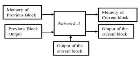
(1) Initialization: The LSTM is initialized off-line from the identification of a classical visual control law. This involves training the parameters of LSTM using data obtained from the classical visual control law in order to establish an initial set of weights and biases (Figure 2).
(2) Online adaptation: An on-line adaptation of the LSTM parameters is implemented to regulate the LSTM's parameters according to the task being performed. This involves updating the weights and biases of the LSTM in real-time based on feedback from the system being controlled, in order to improve the performance of the system as depicted on Figure 3.
Overall, the two steps are essential to implement a control law that involves using a LSTM to regulate the behavior of the system.
where, $S$ is the current value of the visual information, $S_d$ is the desired value, $J^{+}$the pseudo inverse Jacobian matrix of the robot and $T_C$ the camera screw.
Figure 2. Vision control law identification
Figure 3. Revision control law
3.1 LSTM for identification and control
LSTM is suitable for system identification; it models complex system dynamics by capturing temporal input-output dependencies and managing non-linearities [19, 20]. For control, it predicts future states, detects anomalies, and adapts actions based on learned complex system dynamics, involving a comprehensive process from data preparation to real-time implementation. In applications such as robotics control, LSTMs facilitate trajectory prediction, though they require meticulous attention to data quality, computational resources, and model robustness for effective deployment.
In our study, the input to the LSTM is the error between the desired and actual visual features, while the output is the kinematic screw, as illustrated in Figure 2.
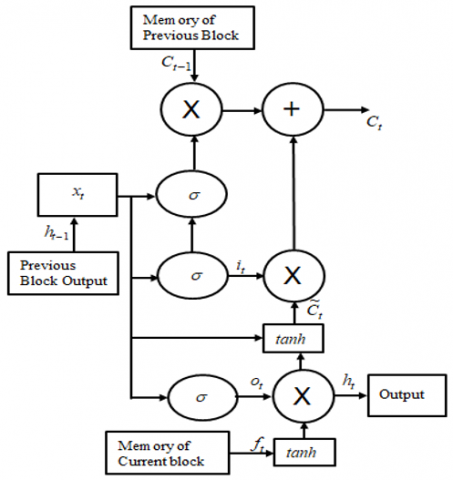
The principle idea of the LSTM is illustrated on Figure 4.
LSTM can remember information for long time, but more previous information may disturb the model accuracy. Typical LSTM module can have three gate activation functions σ. Two output activation functions are hyperbolic tangent functions (tanh) as illustrated in Figure 5.
Figure 4. LSTM principle scheme
Figure 5. LSTM mechanism
where, $h_t$ is the output of the current layer, $h_{t-1}$ denotes the output of the previous layer, $x_t$ the input, $C_t$ the cell state of the current layer, $C_{t-1}$ the cell state of the previous layer, $f_t$ the forget gate layer and $\tilde{C}_t$ the candidate vector.
One can define the system by introducing the forget gate layer given by:
$f_t=\sigma\left(W_{f \cdot}\left[h_{t-1}, x_t\right]+b_f\right)$ (18)
where, $\sigma$ is the sigmoid function, $W_f$ the weights of the forget layer, $x_t$ is the input vector and $b_f$ the bias of the forget layer.
Then, the input layer is updated using the following equations:
$i_t=\sigma\left(W_i \cdot\left[h_{t-1}, x_t\right]+b_i\right)$ (19)
$i_t$ : Is the output of the input gate layer'.
$W_i$ : Is the weights of the input gate layer'.
$b_i$ : Is the bias of the input gate layer'.
$\tilde{C}_t=\tanh \left(W_C \cdot\left[h_{t-1}, x_t\right]+b_C\right)$ (20)
$\tilde{C}_t$: Is the output of the input candidate layer’.
$\tanh$: Is the output of the input candidate layer’.
$W_C$: Is the hyperbolic tangent function.
$b_C$: Is the bias of the candidate layer’.
The output layer is given as follows:
$o_t=\sigma\left(W_o \cdot\left[h_{t-1}, x_t\right]+b_o\right)$ (21)
$o_t$: Is the output of the output gate layer’.
$W_o$: Is the weights of the output gate layer’.
$b_o$: Is the bias of the output gate layer’.
The output of the output gate layer is given by:
$h_t=o_t * \tanh \left(C_t\right)$ (22)
The current cell state can be expressed by:
$C_t=f_t * C_{t-1}+i_t * \tilde{C}_t$ (23)
The proposed configuration for a recurrent neural network (RNN) consists of 3 layers of LSTM cells, with a total of 120 LSTM neurons. The activation function used for the LSTM cell state is set to 'tanh', which is a common choice for RNNs. The activation function used for the LSTM cell gate is set to 'sigmoid', which is also commonly used for this purpose [7, 15].
The hyperbolic tangent function is used as an activation function as depicted by Eq. (24):
$\tanh (x)=\frac{e^x-e^{-x}}{e^x+e^{-x}}$ (24)
where, $e^x$ is the exponential of the input vector.
In order to assess the effectiveness of the proposed control law, experiments using a robot arm of 6 degrees of freedom (UR5) with an attached camera are carried out. The primary goal of these experiments was to track a moving target using the proposed control law, which is capable of detecting and following objects within given scene. The configuration of the system is presented in Figure 6.
Once successfully synthesizing the LSTM based control law, and in order to validate it using Simulink, it was essential to ensure that our simulations were reliable and accurate. To achieve this, the parameters derived from the experimental calibration of the camera module are incorporated, which ensured that the simulated camera mimicked accurately the behavior of the actual camera. Additionally, it has been ensured that the dimensions of the simulated Robot-Camera structure were consistent with those of the real system, which guaranteed the fidelity of the simulated robot's behavior. Following the incorporation of experimental parameters and verification of structural dimensions, we proceeded to evaluate two distinct control structures. The first control structure was designed to facilitate object tracking using a conventional visual servoing control law, which is a widely used technique in the field of robotics. The second control structure focused on tracking a moving object using a robust control law based on Long Short-Term Memory (LSTM) neural networks. This advanced technique is based on recurrent neural networks and has been shown to be highly effective in many robotics applications. Through the evaluation of these two control structures, we were able to compare and contrast their performance and suitability for specific applications.
The proposed scenario is the tracking a desired trajectory as illustrated in Figure 6. To assess the adopted vision control structure, we propose a series of simulations and their corresponding evaluations. The simulation conditions include the following:
Camera module parameters obtained experimentally through a calibration procedure.
UR5 robot dimensions matching those of the real system.
Assumptions made during the simulations:
The object of interest is of point shape.
A set of desired visual coordinates for a single point is used.
The objective of the task is to position the camera relative to the object (a point of interest) such that it aligns with its desired position in the image captured by the camera. The control structure must be designed accordingly, using visual information to manipulate the position and orientation of the camera.
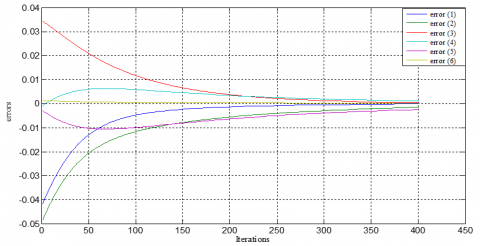
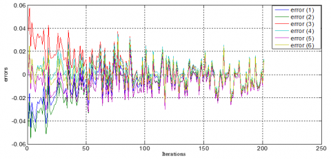
The simulation results are displayed on Figures 7 and 8 for the case of tracking a moving target to test the movement of the robot-camera system based on its 6 degrees of freedom.
On Figure 6, the six components (e(1)-e(6)) of the error values minimized by the visual control law are illustrated, showing successful monitoring of the target. Initially, the error values ranged between [-0.035, 0.048], but after 200 iterations, the error decreased to [-0.003, 0.002], which is an acceptable level of error; corresponding to 0.3%, we can deduce that the precision is 99.7%.
Figure 6. System setup
Figure 7. Control law convergence
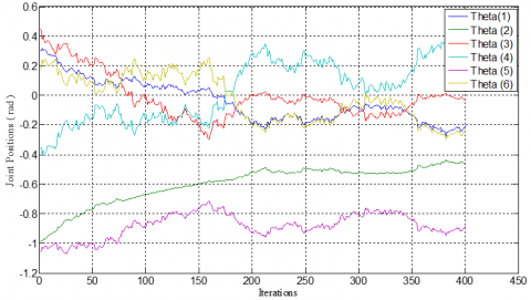
Figure 8. Variations in joint articulations
Figure 8 displays the changes in the joint articulations of the robot as it tracks the movement of the target. During the first 200 iterations, there were significant variations, but after that, Thata (1), Thata (2), and Thata (4) remained fixed, while the last joints exhibited small variations.
4.1 Testing the disturbances rejection and maintaining stability
To evaluate the system's robustness against disturbances and loss of visual features, a test on the conventional visual servoing control law based on the task function is conducted. The test involved adding disturbances and intentionally losing some visual features. The impact of these constraints is illustrated on Figure 9.
Figure 9. Control law convergence in the presence of disturbances
The plot illustrates the error variations in the range of [-0.35, 0.57], which are ten times greater than those without disturbances. However, there are fluctuations in the graph, and the control law is unable to converge.
Figure 10 shows the joint articulation variations of the robot during a tracking task under hard constraints. The plot exhibits jerky movements in all iterations, indicating that the robot is unable to perform the tracking task smoothly.
Figure 10. Joint articulation variations under the influence of disturbances
The previous two figures demonstrated the impact of disturbances on the convergence and joint behavior of the robot. To compare the performance of the proposed control law with the conventional one under the same hard constraints, tests are conducted, and the convergence results are shown on Figure 11.
The error variations in the range of [0, 80] are proportionally greater than those after 80 iterations. This indicates that the proposed control law is capable of rejecting disturbances and compensating the loss of some visual features.
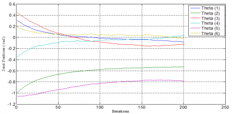
The robust control law proposed in this study demonstrates good performance as evidenced by the smooth plot of the joints positions even under hard constraints, as shown in Figure 12.
Figure 11. Convergence of the robust control law
Figure 12. Variations in joint articulations within the robust control law
The results obtained in the case of a disturbance occurring during the tracking task show that the proposed LSTM control structure allows, on one hand, to control the joint position of the effector. On the other hand, the control signals, although they stabilize and do not show fluctuations. These illustrates the robustness of the control structure with respect to disturbances. However, the curves obtained during the tests showed that the LSTM-based control law has better performance than the conventional visual control law, especially in terms of the speed of convergence. Indeed, the errors in joint tracking exhibit slight oscillations within bounded intervals. This is because LSTM is capable of handling nonlinearity and system complexity.
In this work, a new robust control law for complex systems based on neural networks is proposed. Specifically, LSTM is utilized for both system identification and control of a 6 degrees of freedom UR5 robot manipulator with a camera fixed on its end-effector. The robot's task was to track an object while dealing with hard constraints and loss of some visual features. The obtained simulation results demonstrate that the proposed control law has been successfully validated. The use of LSTM in both identification and control offers superior performance compared to conventional control laws that heavily rely on visual features. Also, the proposed control law can handle situations where some visual features are lost, while conventional control laws may present low performance.
This work makes several original contributions, which are outlined as follows:
However, it is important to note that the proposed control law has certain limitations, which can considered. One remarkable limitation is its inherent inability to effectively compensate or generalize certain scenarios characterized by high-speed visual features, in cases where the object of the interest exhibit rapid movements or possess complex and unpredictable shapes, the control law may struggle to adapt and provide precise control. Similarly, when confronted with objects whose depth varies significantly, the control law may encounter difficulties in maintaining accurate and consistent performance. To address and potentially overcome these limitations, one viable approach involves the implementation of a meta-heuristic algorithm. Such an algorithm could play a pivotal role in optimizing and expediting the learning process of the control law. By using the power of meta-heuristics, the control law could enhance its adaptability and react to a wide range of dynamic and complex scenarios. Furthermore, it is important to note that despite these limitations, the proposed control law remains a valuable tool in industrial automation. Its application extends to various industrial tasks, including but not limited to assembly operations, robotic welding, precision painting and coating tasks, as well as efficient picking and packing processes. In these contexts, the control law can contribute significantly to enhancing productivity, quality, and efficiency, offering a robust solution for a wide array of manufacturing and automation challenges. Overall, the proposed control law offers a promising solution for robust control of complex systems, and further research could explore ways to improve its compensating and generalization abilities.
[1] Huang, W., Zhao, W., Zhang, J. (2019). Visual servo system based on cubature kalman filter and backpropagation neural network. Instrumentation, Mesures, Métrologies, 18(2): 147-151. https://doi.org/10.18280/i2m.180208
[2] Shi, H., Xu, M., Hwang, K.S. (2019). A fuzzy adaptive approach to decoupled visual servoing for a wheeled mobile robot. IEEE Transactions on Fuzzy Systems, 28(12): 3229-3243. https://doi.org/10.1109/TFUZZ.2019.2931219
[3] Wang, Y. (2017). A new concept using LSTM neural networks for dynamic system identification. In 2017 American Control Conference (ACC), IEEE, pp. 5324-5329. https://doi.org/10.23919/ACC.2017.7963782
[4] Wang, J., Zhang, J., Wang, X. (2017). Bilateral LSTM: A two-dimensional long short-term memory model with multiply memory units for short-term cycle time forecasting in re-entrant manufacturing systems. IEEE Transactions on Industrial Informatics, 14(2): 748-758. https://doi.org/10.1109/TII.2017.2754641
[5] Chumakova, E.V., Korneev, D.G., Chernova, T.A., Gasparian, M.S., Ponomarev, A.A. (2023). Comparison of the application of FNN and LSTM based on the use of modules of artificial neural networks in generating an individual knowledge testing trajectory. Journal Européen des Systèmes Automatisés, 56(2): 213-220. https://doi.org/10.18280/jesa.560205
[6] Zhao, Y. (2020). Spatial-temporal correlation-based LSTM algorithm and its application in PM2.5 prediction. Revue d'Intelligence Artificielle, 34(1): 29-38. https://doi.org/10.18280/ria.340104
[7] Liu, N., Li, L., Hao, B., Yang, L., Hu, T., Xue, T., Wang, S. (2019). Modeling and simulation of robot inverse dynamics using LSTM-based deep learning algorithm for smart cities and factories. IEEE Access, 7: 173989-173998. https://doi.org/10.1109/ACCESS.2019.2957019
[8] Rueckert, E., Nakatenus, M., Tosatto, S., Peters, J. (2017). Learning inverse dynamics models in O(n) time with LSTM networks. In 2017 IEEE-RAS 17th International Conference on Humanoid Robotics (Humanoids), IEEE, pp. 811-816. https://doi.org/10.1109/HUMANOIDS.2017.8246965
[9] Galin, R., Meshcheryakov, R., Samoshina, A. (2020). Mathematical modelling and simulation of human-robot collaboration. In 2020 International Russian Automation Conference (RusAutoCon), IEEE, pp. 1058-1062. https://doi.org/10.1109/RusAutoCon49822.2020.9208040
[10] Pollák, M., Kočiško, M., Paulišin, D., Baron, P. (2020). Measurement of unidirectional pose accuracy and repeatability of the collaborative robot UR5. Advances in Mechanical Engineering, 12(12). https://doi.org/10.1177/1687814020972893
[11] Youssef, A., Bayoumy, A.M., Atia, M.R. (2021). Investigation of using ANN and stereovision in delta robot for pick and place applications. International Information and Engineering Technology Association, 8(5): 682-688. https://doi.org/10.18280/mmep.080502
[12] Craig, J. (1989). Introduction to robotics: Mechanics and control (2nd ed.). Canada: Addison-Wesley Publishing Company.
[13] Li, L., Huang, Y., Guo, X. (2019). Kinematics modelling and experimental analysis of a six-joint manipulator. Journal Européen des Systèmes Automatisés, 52(5): 527-533. https://doi.org/10.18280/jesa.520513
[14] Gupta, A., Mondal, A.K., Gupta, M.K. (2019). Kinematic, dynamic analysis and control of 3 DOF upper-limb robotic exoskeleton. Journal Européen des Systèmes Automatisés, 52(3): 297-304. https://doi.org/10.18280/jesa.520311
[15] Zatla, H., Tolbi, B., Bouriachi, F. (2021). Optimal reference trajectory for a type Xn-1Rp underactuated manipulator. Journal Européen des Systèmes Automatisés, 54(3): 503-509. https://doi.org/10.18280/jesa.540314
[16] Djelal, N., Saadia, N., Ramdane-Cherif, A. (2019). Adaptive force-vision control of robot manipulator using sliding mode and fuzzy logic. Automatic Control and Computer Sciences, 53: 203-213. https://doi.org/10.3103/S0146411619030027
[17] Djelal, N., Saadia, N., Ramdane-Cherif, A. (2012). Target tracking based on SURF and image based visual servoing. In CCCA12, IEEE, pp. 1-5. https://doi.org/10.1109/CCCA.2012.6417913
[18] Qasim, M., Ismael, O.Y. (2022). Shared control of a robot arm using BCI and computer vision. Journal Européen des Systèmes Automatisés, 55(1): 139-146. https://doi.org/10.18280/jesa.550115
[19] Ouanane, A., Djelal, N., Bouriachi, F. (2023). Enhanced cardiovascular disease classification: Optimizing LSTM-based model with ant-lion algorithm for improved accuracy. Revue d'Intelligence Artificielle, 37(4): 969-976. https://doi.org/10.18280/ria.370418
[20] Li, T.H.S., Kuo, P.H., Cheng, C.H., Hung, C.C., Luan, P.C., Chang, C.H. (2020). Sequential sensor fusion-based real-time LSTM gait pattern controller for biped robot. IEEE Sensors Journal, 21(2): 2241-2255. https://doi.org/10.1109/JSEN.2020.3016968