Chinedu A. K. Ezugwu*![]() | Ojo S. I. Fayomi
| Ojo S. I. Fayomi![]() | Morakinyo K. Onifade
| Morakinyo K. Onifade![]() | Adeyinka O. M. Adeoye
| Adeyinka O. M. Adeoye![]() | Imhade P. Okokpujie
| Imhade P. Okokpujie![]()
© 2023 IIETA. This article is published by IIETA and is licensed under the CC BY 4.0 license (http://creativecommons.org/licenses/by/4.0/).
OPEN ACCESS
Metal cutting productivity or material removal rate is a constrained objective. Higher productivity, which is guaranteed by higher cutting process parameters (feed, speed, and depth of cut), is accompanied by higher constraining and unwanted factors like higher cutting forces, higher power demand, higher machine tool and workpiece deflections (in other words, form error), higher waste heat generation and coolant demand, faster tool wear rate, higher predisposition to periodic and regenerative chatter, compromised surface quality, etc. The research focused on the development of theoretical and numerical framework for selecting the cutting process parameters to enhance the productivity, integrity, and accuracy of turned slender parts. The method involved theoretical modelling that expresses material removal rate and form error in terms of cutting process parameters, workpiece flexibility parameters, workpiece geometrical parameters, and kinematic parameters. Cutting tests were carried out in validation of the arising theoretical and numerical results. Parametric studies were carried out using the developed computational model to understand the trend of accuracy and productivity with variation of cutting process parameter. As expected, the parametric study shows that flexibility of the slender workpiece reduced MRR. The results showed that deviation of predicted values of MRR from the desired values rises with rise of all the cutting process parameters; feed, depth of cut and spindle speed. The findings also indicate that as the feed rate and depth of cut increase, the variance between the predicted diameter and the target values also increases. However, there is a fluctuating pattern with a gradual decrease in variance as the spindle speed rises. Based on the results of the parametric studies, specified tolerance ranges could be met by choosing parameter sets that meet the specifications. If the numerical model relies on FEA, it might require extensive computational resources and expertise, limiting its practicality. Overcoming these limitations often involves continuous research and development efforts, incorporating real-world data, and improving the accuracy and adaptability of the framework for specific machining scenarios. The parametric study results can be used as a framework for the selection of cutting process parameter to enhance the productivity, integrity, and accuracy of turned slender parts.
computational modelling, material removal rate, flexibility, accuracy, productivity
Slender workpieces still present a technological challenge during turning on the lathe because of their low damping and stiffness [1]. As a result of low stiffness, they are prone to form error while as a result of low damping, they are prone to different types of chatter vibrations. A vibration model based on workpiece compliance and rigid machine tool clamping system was validated by workpiece vibration and cutting force measurements in two perpendicular directions. The novel experimental method, which was on the basis of the variations in the computed workpiece natural frequencies when cutting is involved and when cutting is not involved was demonstrated to be useful for ascertaining the cutting damping ratio [2, 3]. The applied cutting force equation comprised terms that were directly related to the workpiece’s displacement and its velocity along the tool axis. The innovative experimental method proposed in the work was found to be convenient for measuring the damping ratio of long slender workpieces during turning processes. A technique for modelling the relationships between the machine tool structure and cutting process and the effects on dynamic stability and dynamics control was established using stochastic modelling [4-6]. The authors found that as long as the studied system remains within the stable operational range that estimations of frequency and damping factor using the developed control system are less than 6% which is acceptable under dynamic machining conditions. In the works [7, 8], the various sources of geometric errors of machined parts and the traditional methods of compensating or eliminating the errors were presented with a briefcase study of cutting-force induced errors. The errors sources in machined parts which have allusions of errors due to the response of workpiece or machine tool structures were summarized by the authors to include: geometric errors of machine structures and parts, and kinematic errors, thermal distortions errors, errors induced by forces like gravity loads, inertial effects of axes, cutting forces, tool wear, fixture, instrumentation errors, tool wear errors, machine assembly-stimulated errors, fixture errors, material instability errors and others. In the opinion of the work [9], excessive deformations that cause form error and chatter vibrations constitute the major barriers regularly stumble upon in turning of long flexible workpieces. A new technique for optimally selecting machining process parameters and sequence of cutting passes to control chatter and deformation in the turning of a slender rod was introduced in the work. With cutting time as the objective function and with the deformation due to workpiece flexibility and regenerative chatter as the constraints, they solved the optimization problem in two phases. While the first phase employed a combination of sequential quadratic programming technique and genetic algorithm to decide the minimum production time for one cutting pass with specified cutting depths, the second phase employed the dynamic programming technique to find the optimum sequential subdivision of the total cutting depth. As pointed out in the studies [1, 9-12], the flexibility of workpiece, and the associated surface location error, has not been comprehensively considered with regard to the turning and other lathe operations for the machining of slender workpieces. The semi-discretization method was used to analyse a delayed flexible multi-body model of a thin-walled workpiece processed by turning process [13, 14]. The investigators used an adaptronic tool holder made up of sensors and actuators to suppress dynamic instability. The control concept was aimed at tuning the active system to improve the region of stable cutting and it was found that the stability boundary can be significantly enhanced.
Orthogonal turn-milling is a primary technique in machining. It is typically employed for challenging materials, large rotary components, slender rods, and thin-walled rotary parts. However, in the realm of milling and turning operations, orthogonal turn-milling can lead to the occurrence of chatter, which has been observed to impact machining efficiency, precision, and tool longevity. Several methods have been developed in the effort to predict chatter stability in orthogonal turn-milling. These approaches include full-discretization, semi-discretization, zero-order analytical, multi-frequency solution, temporal finite element analysis, and these methods. The complexity of orthogonal turn-milling in the real world may not be sufficiently accounted for by the zero-order analytical method, it should be noted. Similar to this, the full-discretization strategy necessitates complex iterative equations and only achieves partial discretization, in contrast to the multi-frequency solution, temporal finite element analysis, and semi-discretization methods. In order to address these difficulties, Sun et al. [15] introduced a fresh stability model for orthogonal turn-milling. The model utilized a comprehensive discretization approach to analyze the cutting process in orthogonal turn-milling and generated stability-lobe diagrams. Furthermore, the validation of the diagrams was carried out using the experimental results. The feeding per revolution of tools influence on cutting stability was analyzed and reported in this work. In conclusion, they suggested that the theoretical model put forward has the potential to offer valuable guidance for optimizing both the efficiency of the machining process and the surface quality of workpieces produced through orthogonal turn-milling, as discussed in reference [15]. In the study [16], they employed the Newton iterative approach to develop both a compensation method and an influence analysis technique for addressing geometric errors. These errors were based on the homogeneous coordinate transformation matrix. The approach involved integrating an error matrix into the kinematic model of a four-axis machine tool to assess how each axis’s geometric error affected the tool’s path. The proposed method defined geometric errors using a homogeneous coordinate transformation matrix and proceeded to construct a comprehensive geometric error compensation calculation model through Newton iteration. This model factored in the machine’s four-axis kinematic model while considering geometric errors. To validate this method, they conducted experiments with a four-axis machine tool, using a curved tool path for an off-axis optical lens. The outcomes demonstrated that the suggested technique can greatly increase machining accuracy.
According to Woźniak and Parus [17], the idea of using a controlled vibration eliminator to lessen vibrations produced while turning has been put forth. The workpiece that the active holder is supporting has the eliminator incorporated in it. The components of a mechatronic system model are a workpiece, a hydraulic actuator, and the machining operation. Turning long slender object was simulated using a model of the system. Simulated machining operations with and without vibration eliminators were provided with their outcomes. The designed system was determined to be able to reduce vibration amplitude and boost vibration stability throughout the turning process based on the simulation. The suppression of chatter when time-periodic axial pressure was applied when rotating slender workpieces was examined in the study by Beri et al. [18]. The mathematical model of the workpiece that was pinned at the tailstock and clamped at the chuck was built using the Euler-Bernoulli beam theory. To enhance the stability of the turning process, the workpiece is subjected to a cyclic compressive force featuring various waveforms, including sinusoidal, triangular, and square-shaped patterns. These modulations, which were caused by the induced time-periodic fluctuation of the workpiece’s lateral stiffness, result in complex patterns in the stability chart. Their research shown that turning, a practical alternative for low cutting speeds, considerably benefits from the modification of the axial force in a multi-dimensional parameter space.
Sekar et al. [19] examined the impacts of deflections in a workpiece supported by a tailstock and introduced a compliant dynamic cutting force model with two degrees of freedom. The relative motion between the workpiece and the cutting tool serves as the foundation for this model. This work observed that in the process of cutting a slender and flexible work piece at high speeds, the critical chip width is larger than a rigid work piece. In conclusion, this dynamic model examined how the dynamic stability was affected by the cutting position, workpiece dimensions, cutter flexibility, and cutter damping. In order to speed up production and cut costs, Gururaja et al. [20] published an examination of the viability of utilizing a numerical method to determine the modal parameters for various machining settings. For the purpose of predicting stable process parameters, an experimentally produced stability lobe diagram considers the impact of variable stiffness. After conducting an experimental modal analysis on a flexible, thin-walled Ti6Al4V material, the obtained modal characteristics were subjected to experimental verification. The results of this validation process revealed a 5.1% discrepancy in the predicted natural frequency and an 8.04% variation in the expected modal stiffness. The selection of stable parameters based on the stiffness-dependent stability lobe is expected to enhance the cutting tool’s longevity and boost material removal rates. Urbikain et al. [21] made stability predictions in the context of straight turning with a flexible workpiece. They accomplished this by introducing an algorithmic model based on the Chebyshev collocation method. Their Single Degree of Freedom (SDoF) model incorporated various factors, including tool lead angle, cutting speed, round inserts, and depth of cut. Subsequently, they utilized ANSYS software to perform finite element analysis (FEA) on a model of the workpiece with a concentrated mass. The model proved to be valuable for low-order stability lobes, accurately predicting stability up to 87.5%. However, there were inconsistencies because of problems with modeling and the model’s input parameters, such as cutting coefficients and modal parameters. It’s important to note that several earlier researches also looked at the compliance of the tool-workpiece system. According to these authors, taking tool-workpiece compliance into account is essential for developing a more accurate model. Guo et al. [22] explored the influence of tool setting on the form error in MLA (Micro Lens Array) manufacturing and proposed a novel two-step tool setting strategy for UPDT (Ultra-Precision Diamond Turning) in their research. Initially, they established a theoretical model to describe form errors in MLA resulting from tool setting inaccuracies. To address these errors in tool setup, they devised an innovative two-step method. Subsequently, they conducted multiple experiments involving MLA fabrication with varying tool setting errors and assessed the resulting from errors. Both the theoretical and practical outcomes demonstrated that the proposed tool setting approach offers high precision accuracy. It was also revealed that tool setting errors could significantly introduce periodic form imperfections in the MLA during UPDT. Importantly, this study contributes to a deeper understanding of the impact of tool setting on the form accuracy of MLA in UPDT, with potential for further advancements in this area. Yu et al. [23] investigated how sliding and dynamic errors impact the accuracy of micro-structured surfaces machined with diamond turning. In parallel, Liu et al. [24] introduced a multi-body system (MBS) model for a three-axis ultra-precision lathe and explored how geometric errors influenced coordinate distortion and form accuracy. Their study emphasized that achieving better surface quality relied on identifying and accurately rectifying the primary errors affecting the machining process [25]. These high-quality machined surfaces could be designed to control the direction of light propagation, effectively eliminating diffraction effects, and offering a qualitative analysis of optical component performance and improvements [26]. To identify the dominant errors affecting machining accuracy, a common approach involved removing the workpiece for offline measurement [27-30]. In this context, a measurement technique based on the double ball bar (DBB) was proposed to address geometric error measurement challenges for five-axis ultra-precision machine tools operating with interpolated five-axis motion [31]. Their suggested method was less constrained by the machine tool’s configuration and could measure the geometric errors of a five-axis ultra-precision machine tool with a single setup. The measurement procedure involved planning a motion trajectory, ensuring that the DBB’s length remained constant during the measurement process. Additionally, the hypothesized outcomes of the error model were contrasted with the measured results. It was discovered that the measurement data’ trend and amplitude match the conclusions from theory.
Nagayama and Yan [32] in their work considered a deterministic process in determining and compensating machine tools error by proposing a model that possess all the main error factors. They opined that offline measurement also gives high identification accuracy, but they noted that it has its own drawbacks such as breaking the continuity of cutting and low working efficiency. In traditional manufacturing processes, it is crucial to give due attention to real-time error measurements. Online error measurements can be conducted by employing 3D topography surface analysis, but it is essential to seamlessly integrate the measurement equipment into the system. This integration ensures the identification and compensation of tool errors [33-36]. The work of Li et al. [37] was able to identify and compensate for motion errors by proposing an online measurement method that integrated the interferometric surface metrology into the machine tool. In their research, Tong et al. [38] enhanced the precision of tool alignment by incorporating embedded probes and successfully achieved on-machine measurements of FTS machined surfaces. They observed that challenges like lubricant splattering and chip adhesion during machining can negatively impact the performance of sensors like optical lenses and probes. Consequently, they suggested the adoption of displacement sensors and dynamometers to enhance methods for identifying machining errors and machine tool inaccuracies.
Effort on improving non-circular turning accuracies are mentioned by various authors, Hu et al. [39] proposed a unique control structure that recognizes form errors as a direct objective. They used real-time form error analysis in their research. They proposed an online control technique focused on correcting the motion commands of the fast-radial servo motor in an effort to reduce form errors. This method involved the decoupling of control loops for individual drives, concentrating only on fast-radial servo drive compensation of position commands without changing the inner velocity and current loops. They argued that this novel strategy outperformed the conventional contouring error control structure, which depended on cross-coupled compensations for all axes, in terms of effectiveness. Additionally, they tested their internally developed non-circular turning prototype to validate the model’s predictions. They observed that as compared to conventional controllers, which mainly focused on individual drive tracking error management, their error estimation and compensation methods greatly improved contouring accuracy. Yang et al. [40] investigated a mechanism that utilized a two-degree tool holder. In their study, they employed a distinct trajectory interpolation algorithm that involved changing spindle speed while maintaining a consistent tangential feed rate. The experimental outcomes revealed reduced fluctuations in cutting loads and improved tracking and contour accuracy in comparison to the conventional approach of using a constant spindle speed. This method was noted to be more effective than that of traditional method.
To increase the productivity, integrity, and precision of turned slender components, a theoretical and numerical framework for choosing the cutting process parameters has been developed in this research. Using theoretical modelling, the approach expressed material removal rate and form error in terms of cutting process parameters, workpiece flexibility parameters, workpiece geometrical parameters, and kinematic parameters. The emerging theoretical and numerical results were validated using cutting experiments. To understand the trend of accuracy and productivity with variation of cutting process parameter, parametric studies were conducted using the established computational model. This is novel in the area of machining and will guide machinist in selecting appropriate parameters for better productive and accuracy.
Machining efficiency is measured by considering machining time, material removal rate, and the economics of machining. To put it simply, the overall machining time or the total time for machining (Tm) is the sum of all three individual time components that are directly associated with the machining process, as indicated in reference [41].
The time components are listed below:
Arithmetically, the complete Time for Machining (Tm) may be expressed as:
$\mathrm{T}_{\mathrm{m}}=\mathrm{T}_{\mathrm{ct}}+\mathrm{T}_{\mathrm{i}}+\mathrm{T}_{\mathrm{c}}$ (1)
If we denote s as the feed rate in millimeters per revolution, Lc as the total cutting length in millimeters, and Ω as the spindle speed in revolutions per minute (rpm), we can express the suggested cutting time as follows:
$\mathrm{T}_{\mathrm{c}}=\frac{L_c}{\Omega . s}$ (2)
Traditionally, when either the workpiece or the cutting tool is in motion, the spindle speed and cutting speed ($V_c$) are often used interchangeably. This assumption is made under the premise that there is no speed loss between the spindle and workpiece for the cutting operation. However, it's important to note that cutting speed is also influenced by the size of the workpiece or cutter (D). Consequently, we can express cutting speed as a function of diameter as follows:
$V_c=\frac{\pi D \Omega}{1000}$ (3)
Then,
$T c=\frac{\mathrm{L}_{\mathrm{s}}}{\Omega . \mathrm{s}}=\frac{\mathrm{L}}{\left(\frac{1000 \mathrm{~V}_{\mathrm{c}}}{\pi \mathrm{D}}\right) \mathrm{s}}=\frac{\pi \mathrm{DL}}{1000 \mathrm{~V}_{\mathrm{c}} \mathrm{s}}$ (4)
The Expression for Taylor’s Tool Life is:
$V_c(T L)^n=C$ (5)
$\mathrm{TL}=\left(\frac{C}{V_c}\right)^{1 / n}$ (6)
Considering tool life in the calculation of total machining time is essential for optimizing machining processes, reducing costs, and improving overall manufacturing efficiency. It allows manufacturers to strike a balance between minimizing tooling expenses and maximizing productivity while maintaining product quality.
Conversely, the total machining setup time (Tct) is also influenced by the extent of the desired adjustments, and the lifespan of the tool will affect this time component. Therefore, if TCT represents the time required for a single tool change, the total machining setup time (Tct) for the entire machining operation with a length of Tct can be expressed as follows:
$T_{c t}=\frac{T_c}{T L} \times T C T$ (7)
As a result, the comprehensive machining time or the total time for machining can be expressed in the following manner:
$\begin{gathered}\mathrm{T}_{\mathrm{m}}=\mathrm{T}_{c . t}+\mathrm{T}_{\mathrm{i}}+\mathrm{T}_c \end{gathered}$ (8)
$ T m=T c+\frac{T_c}{T L} \times T C T+T i $ (9)
$\mathrm{Tm}=\frac{\pi D L}{\left(1000 V_c\right) s}+\left\{\frac{\frac{\pi D L}{\left(1000 V_c\right) s}}{\left(\frac{C}{V_c}\right)^{1 / n}} \times T C T\right\}+\mathrm{Ti}$ (10)
$ \mathrm{Tm}=\frac{\pi D L}{\left(1000 V_c\right) s}+T C T \frac{\pi D L}{1000 s C^{1 / n}} V_c^{\frac{1-n}{n}}+T_i$ (11)
This investigation’s main focus is on how long the actual machining takes. Many research projects do not see the actual machining time as their only goal, but rather as a predictor of both the surface quality and the rate of material removal. For instance, the study by Qehaja et al. [42] investigated the relationship between surface roughness (Ra) and the parameters for machining, which encompass factors like the extent of material removal, the curvature of the cutting tool’s tip, the effective rake angle, the velocity of the cutting tool, the actual machining duration, the rate of material feed, and the angle of the cutting tool’s side edge. They utilized response surface techniques and a three-tiered factorial design to construct a practical model for surface roughness, considering aspects such as tool design, the time spent on machining, the curvature of the cutting tool’s tip, and the material feed rate during dry turning operations.
The techniques involved in simulating the statically reactive behavior of a flexible workpiece to the thrust component of the cutting forces were applied. The study examined the effects of the beam-models’ reactions on the pace of material removal and the degree to which the actual form and size departed from the desired specifications. This investigation covered two separate scenarios, one in which the workpiece was shown as a cantilever and the other as a fixed-pinned beam. You can find the equations characterizing the deflections of the fixed-pinned beam [43, 44] in Figure 1, which appropriately depicts the model for a flexible workpiece supported by both the chuck and the tailstock center.
$ R_1=\frac{F b}{2 l^3}\left(3 l^2-b^2\right)=V_{A B}$ (12)
$R_2=\frac{F a^2}{2 l^3}(3 l-a)=-V_{B C}$ (13)
$M_1=\frac{F b}{2 l^2}\left(b^2-l^2\right) $ (14)
$ M_{A B}=\frac{F b}{2 l^3}\left(b^2 l-l^3-x\left(3 l^2-b^2\right)\right) $ (15)
$ M_{B C}=\frac{F a^2}{2 l^3}\left(3 l^2-3 l x-a l+a x\right) $ (16)
$ y_{A B}=\frac{F b x^2}{12 E I l^3}\left(3 l\left(b^2-l^2\right)+x\left(3 l^2-b^2\right)\right) $ (17)
$ y_{B C}=y_{A B}-\frac{F(x-a)^3}{6 E I}$ (18)
Figure 1. The slender workpiece supported by the chuck and tailstock centre is modelled as a fixed-pinned beam deflection
The model shown in Figure 2, which is adequate for a slender workpiece supported by the chuck alone, contains equations for the deflections of the cantilever beam [43, 44].
$R_1=V=F $ (19)
$ M_1=-F a $ (20)
$ M_{A B}=F(x-a) $ (21)
$ M_{B C}=0 $ (22)
$ y_{A B}=\frac{F x^2}{6 E I}(x-3 a) $ (23)
$ y_{B C}=\frac{F a^2}{6 E I}(a-3 x)$ (24)
Figure 2. Model of a thin workpiece held solely by the chuck using a cantilever beam
In order to illustrate the machining issue under examination, these equations were then transformed, and used to analyse how workpiece flexibility affected cutting forces, as well as how it affected precision and the pace at which material was removed.
The cutting force has three components, Figure 3 the tangential force $F_{c, \text { sum }}$, the feed force $N_{c, \text { sum }}$ and the thrust force $F_{t h, \text { sum }}$. The feed force $N_{c, \text { sum }}$ acts in compressive mode in the axial direction. Since the workpiece is much stronger in the axial compressive mode that flexural mode and the fact that any compression in the axial direction will not necessarily influence dimensional integrity, the effects of the feed force are normally neglected. The tangential force $F_{c, \text { sum }}$ will have a torsion effect which will not affect much the material removal rate and final dimensional integrity, the effects of the force are also normally neglected.
In the context of machining and manufacturing processes, various assumptions are made regarding workpiece material, cutting conditions, and machine tool stiffness to simplify the analysis and modelling. These assumptions help in creating theoretical frameworks and numerical simulations for practical applications. Here are some of the assumptions made in this research: The material properties, such as Young’s modulus, Poisson’s ratio, and thermal conductivity, were assumed to be constant and not affected by factors like temperature, strain, or stress, steady-state cutting conditions was assumed, where cutting forces, temperatures, and tool wear reach a relatively constant level over time, the workpiece was assumed to be perfectly clamped or fixtured, without any vibration or movement during machining and machine tools were assumed to be rigid and not subject to deflection or deformation during the machining process.
The thrust force $F_{t h, s u m}$, which acts perpendicular to the spindle axis, tend to deflect the workpiece. The thrust force $F_{t h, s u m}$ is the radial component of the cutting force which is due to the nose radius and non-zeros approach angle $\vartheta$ (see Figure 4).
Figure 3. The cutting force system
Figure 4. Turning process showing nose radius and non-zeros approach angle $\vartheta$ which induces the thrust force $F_{t h}$
During turning of flexible workpiece supported by the chuck and the tailstock centre (henceforth, called Model 1 sometimes) or a workpiece fixed at the chuck and free at the other end (henceforth, called Model 2 sometimes). Eqs. (12) to (24) apply such that:
$F=F_{t h, s u m}$ (25)
Assuming that a cutting pass proceeds such as to approach the headstock then machined distance b becomes:
$b=v t$ (26)
and
$a=l-v t$ (27)
where, l is the length of the workpiece. The material removal rate is given as:
$\operatorname{MRR}(a)=\rho w(a) h V_t$ (28)
where, $\rho$ is the density of the workpiece material in $\mathrm{kgm}^{-3}$, $w(a)$ is the actual depth of cut as a function of workpiece deflection at $x=a$. The actual depth of cut $w(a)$ is the remainder when the deflection is deducted from the intended depth $w$. Therefore:
$w(a)=w-\left|y_{A B}(a)\right|$ (29)
where for Model 1:
$y_{A B}(a)=\frac{F b a^2}{12 E I l^3}\left(3 l\left(b^2-l^2\right)+a\left(3 l^2-b^2\right)\right)$ (30)
and for Model 2:
$y_{A B}=-\frac{F a^3}{3 E I}$ (31)
The deflections are written in terms of the instantaneous machining time. For Model 1, this becomes:
$\begin{gathered}y(t)=\frac{F_{\text {th }, \text { sum }}}{12 E I l^3} v t(l-v t)^2\left(3 l\left(v^2 t^2-l^2\right)+\right. \left.(l-v t)\left(3 l^2-v^2 t^2\right)\right)\end{gathered}$ (32)
which is simplified to:
$y(t)=\frac{-F_{t h, s u m}}{12 E I l^3} v^2 t^2(l-v t)^3(3 l+v t)$ (33)
For Model 2 the time-dependent deflection is:
$y(t)=-\frac{F_{t h, s u m}(l-v t)^3}{3 E I}$ (34)
The instantaneous depths of cut, now expressed as a function of time, for Model 1 and Model 2 will respectively become.
$w(t)=w-\frac{F_{t h, s u m}}{12 E I l^3} v^2 t^2(l-v t)^3(3 l+v t) $ (35)
$ w(t)=w-\frac{F_{t h, s u m}(l-v t)^3}{3 E I}$ (36)
It should be noted that the thrust force $F_{t h, s u m}$ is now also a function of time as follows:
$F_{t h, s u m}(t)=K_{t h} h w(t)+K_{t h, e} w(t)$ (37)
For Model 1, this becomes:
$\begin{gathered}F_{t h, s u m}(t)=\left(K_{t h} h+K_{t h, e}\right) w+\left(K_{t h} h+\right. \left.K_{t h, e}\right) \frac{F_{t h, s u m}(t)}{12 E I l^3} v^2 t^2(l-v t)^3(3 l+v t)\end{gathered} \\ \begin{gathered}F_{t h, \text { sum }}(t)\left(1-\frac{\left(K_{t h} h+K_{t h, e}\right)}{12 E I l^3} v^2 t^2(l-v t)^3(3 l+\right. v t))=\left(K_{t h} h+K_{t h, e}\right) w\end{gathered} \\ F_{t h, s u m}(t)=\frac{\left(K_{t h} h+K_{t h, e}\right) w}{\left(1-\frac{\left(K_{t h^{h+K}} t h, e\right.}{12 E I l^3} v^2 t^2(l-v t)^3(3 l+v t)\right)}$ (38)
Eq. (35) therefore, becomes:
$w(t)=w-\frac{\left(K_{t h} h+K_{t h, e}\right) w v^2 t^2(l-v t)^3(3 l+v t)}{\left(12 E I l^3-\left(K_{t h} h+K_{t h, e}\right) v^2 t^2(l-v t)^3(3 l+v t)\right)}$ (39)
For Model 2, this Eq. (37) becomes:
$\begin{gathered}F_{t h, s u m }(t)=\left(K_{t h} h+K_{t h, e}\right) w+\left(K_{t h} h+\right. \left.K_{t h, e}\right) \frac{F_{t h, s u m}(t)(l-v t)^3}{3 E I}\end{gathered} \\ \begin{gathered}F_{t h, s u m}(t)\left(1-\left(K_{t h} h+K_{t h, e}\right) \frac{(l-v t)^3}{3 E I}\right)=\left(K_{t h} h+\right. \left.K_{t h, e}\right) w\end{gathered} \\ F_{t h, s u m}(t)=\frac{\left(K_{t h} h+K_{t h, e}\right) w}{\left(1-\left(K_{t h} h+K_{t h, e}\right) \frac{(l-v t)^3}{3 E I}\right)}$ (40)
Eq. (36) for Model 2 therefore, becomes:
$w(t)=w-\frac{\left(K_{t h} h+K_{t h, e}\right) w(l-v t)^3}{\left(3 E I-\left(K_{t h} h+K_{t h, e}\right)(l-v t)^3\right)}$ (41)
The material removal rate, now seen as a function of time, respectively becomes:
$\begin{gathered}\operatorname{MRR}(t)=\frac{\rho \pi D}{60} h \Omega \mathrm{w}+ \frac{\rho \pi D}{60} h \Omega \frac{\left(K_{t h} h+K_{t h, e}\right) w v^2 t^2(l-v t)^3(3 l+v t)}{\left(12 E I l^3-\left(K_{t h} h+K_{t h, e}\right) v^2 t^2(l-v t)^3(3 l+v t)\right)}\end{gathered}$ (42)
$\begin{gathered}\operatorname{MRR}(t)=\frac{\rho \pi D}{60} h \Omega \mathrm{w}+ \frac{\rho \pi D}{60} h \Omega \frac{\left(K_{t h} h+K_{t h, e}\right) w(l-v t)^3}{\left(3 E I-\left(K_{t h} h+K_{t h, e}\right)(l-v t)^3\right)}\end{gathered}$ (43)
For Model 1 and Model 2. The total amount of material removed now becomes:
$m=\int_0^{l / v} \operatorname{MRR}(t) d t$ (44)
For Model 1 this reads:
$\begin{gathered}m=\frac{\rho \pi D l}{60} \frac{h \Omega \mathrm{w}}{v}+ \frac{\rho \pi D}{60} h \Omega \int_0^{l / v} \frac{\left(K_{t h} h+K_{t h, e}\right) w v^2 t^2(l-v t)^3(3 l+v t)}{\left(12 E I l^3-\left(K_{t h} h+K_{t h, e}\right) v^2 t^2(l-v t)^3(3 l+v t)\right)} d t\end{gathered}$ (45)
and Model 2 this reads:
$\begin{gathered}m=\frac{\rho \pi D l}{60} \frac{h \Omega \mathrm{w}}{v}+ \frac{\rho \pi D}{60} h \Omega \int_0^{l / v} \frac{\left(K_{t h} h+K_{t h, e}\right) w(l-v t)^3}{\left(3 E I-\left(K_{t h} h+K_{t h, e}\right)(l-v t)^3\right)} d t\end{gathered}$ (46)
The integrations cannot readily be evaluated analytically; therefore, they will be evaluated numerically using either the composite trapezoidal rule or the composite Simpson’s rule.
The intended diameter of the machined part is $D-2 w$ but because of flexibility, the compromised diameter becomes $D(t)=D-2 w(t)$ which for Model 1 becomes:
$\begin{gathered} D(t)=D-2 w+ 2 \frac{\left(K_{t h} h+K_{t h, e}\right) w v^2 t^2(l-v t)^3(3 l+v t)}{\left(12 E I l^3-\left(K_{t h} h+K_{t h, e}\right) v^2 t^2(l-v t)^3(3 l+v t)\right)}
\end{gathered} $ (47)
and for Model 2 becomes:
$D(t)=D-2 w+2 \frac{\left(K_{t h} h+K_{t h, e}\right) w(l-v t)^3}{\left(3 E I-\left(K_{t h} h+K_{t h, e}\right)(l-v t)^3\right)}$ (48)
The average diameter can be evaluated for either of the models from solving the equation.
$\overline{\mathrm{D}}=\frac{v}{l} \int_0^{l / v} \mathrm{D}(t) d t$ (49)
For Model 1 this reads:
$\begin{gathered}\overline{\mathrm{D}}=D-2 w+ 2 \int_0^{l / v} \frac{\left(K_{t h} h+K_{t h, e}\right) w v^2 t^2(l-v t)^3(3 l+v t)}{\left(12 E I l^3-\left(K_{t h} h+K_{t h, e}\right) v^2 t^2(l-v t)^3(3 l+v t)\right)} d t\end{gathered}$ (50)
and Model 2 this reads:
$\overline{\mathrm{D}}=D-2 w+2 \int_0^{l / v} \frac{\left(K_{t h} h+K_{t h, e}\right) w(l-v t)^3}{\left(3 E I-\left(K_{t h} h+K_{t h, e}\right)(l-v t)^3\right)} d t$ (51)
In the above presented equations $h=f \cos (\vartheta)$ is the chip thickness where $f$ is the feed.
Over time, data from deflection models can be used to identify trends and areas for process improvement. By analysing the accumulated data, you can refine machining strategies and improve the overall manufacturing process. In summary, deflection models for flexible workpieces are valuable tools for optimizing machining processes and achieving greater precision in real-world manufacturing settings. These models, when properly integrated and applied, can lead to reduced waste, improved product quality, and increased efficiency in machining operations.
The equations developed are simulated using the numerical values of the thrust force coefficients drawn from Hanif et al. [45] and the analytical methodology for calibration of force coefficients from force data was used to give the thrust force coefficients as:
$\begin{gathered}K_{t h}=4.5245 \times 10^8 \mathrm{Nm}^{-2} \quad \text { and } \quad K_{t h, e}=0.0005 \times 10^8 \mathrm{Nm}^{-1} .\end{gathered}$
The parameters $v=0.0025 \mathrm{~ms}^{-1}, w=1.5 \mathrm{~mm}$ and $\Omega=500 \mathrm{rpm}$ are typical in turning processes. Let a workpiece length $l=0.5 \mathrm{~m}$ and aluminium with typical tensile modulus $E=70 \mathrm{GPa}$, density $\rho=2650 \mathrm{kgm}^{-3}$ be assumed. A typical diameter $D=30 \mathrm{~mm}$ is assumed for a slender workpiece. The chip thickness becomes $h=f=v \frac{60}{\Omega}=3 \times 10^{-4} \mathrm{~m}$. The polar moment of inertia therefore becomes $I=\pi \frac{D^4}{32}=$ $7.9522 \times 10^{-8} \mathrm{~m}^4$.
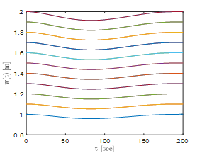
By employing Eq. (39) within the framework of Model 1, we conducted a simulation to depict the fluctuation of the instantaneous depth of cut, $w(t)$, with respect to time $t$ and its location a from the fixed end (chuck). This simulation is illustrated in Figure 5, focusing on a designated depth of cut, $w=1.5 \mathrm{~mm}$. The graph clearly shows that the depth of cut fluctuates, periodically reducing and increasing, yet it consistently remains below the specified depth of cut. It is evident from the figure that both the point in time and the specific location where the depth of cut reaches its minimum can be readily determined from the plots. To investigate how the prescribed depth of cut, w, affects the behavior of the instantaneous depth of cut, $w(t)$, we conducted simulations for various prescribed depths of cut, ranging from $w=1.0 \mathrm{~mm}$ to $w=2.0 \mathrm{~mm}$, as presented in Figure 6 . Notably, a decrease in the prescribed depth of cut leads to a reduction in the variation of the instantaneous depth of cut.
Figure 5. A change in the instantaneous depth of cut, denoted as w(t), over time t and at a specific position a relative to the fixed end (chuck) for Model 1
Figure 6. A variation of instantaneous depth of cut $w(t)$ with time $t$ for several prescribed depths of cut from $w=1.0 \mathrm{~mm}$ to $w=2.0 \mathrm{~mm}$ for Model 1
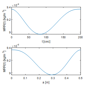
Figure 7. A variation of instantaneous material removal rate $\operatorname{MRR}(t)$ considering time t and the position a relative to the fixed end (chuck) for Model 1
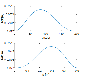
Figure 8. A change in the workpiece’s diameter, denoted as D(t), over time t and at a specific position a relative to the fixed end (chuck) for Model 1
Using Eq. (28) for Model 1, a variation of instantaneous material removal rate $\operatorname{MRR}(t)$ with time $t$ and location $a$ is plotted in Figure 7 for a prescribed depth of cut $w=1.5 \mathrm{~mm}$. It can be seen that material removal rate has similar trend as the instantaneous depth of cut. This means that the prescribed depth of cut has similar effect on $\operatorname{MRR}(t)$ as $w(t)$.
Using Eq. (47) for Model 1, a variation of instantaneous diameter of the machined part of the workpiece $D(t)$ with time $t$ and location $a$ is simulated and plotted in Figure 8. It must be noted that the diameter of the machined part should be $D-$ $2 w=30-3=27 \mathrm{~mm}$. It is obvious from the figure that because of workpiece flexibility, diameter increases and reduces but stays greater than the prescribed machined diameter of $27 \mathrm{~mm}$. It can be seen from the figure that both the time and location at which diameter maximizes can easily be read from the plots and applied in tolerance analysis.
Using the data of Figure 7 and applying the composite trapezoidal rule to Eq. (44), the total amount of material removed can be computed. The composite trapezoidal rule adapted to this case is given as:
$\begin{gathered}m=\frac{\Delta t}{2} \operatorname{MRR}\left(t_0\right)+\Delta t \sum_{k=1: 1: K-1} \operatorname{MRR}\left(t_k\right)+ \frac{\Delta t}{2} \operatorname{MRR}\left(t_K\right)\end{gathered}$ (52)
where, $t_k$ is a discrete time. Applying this equation, the actual mass of material removed becomes estimated as $m=$ $0.1835 \mathrm{~kg}$. The expected value in the absence of flexibility is $m=\rho l \frac{\pi\left(D^2-(\mathrm{D}-2 w)^2\right)}{4}$. Therefore, $m=0.1780 \mathrm{~kg}$ is expected. Though the actual and the expected values are close, the trapezoidal rule over-estimates the actual material removed since it is expected to be less than the expected value. This is due to inability of the trapezoidal rule to capture the steeper slope of the deflection curve for higher depths of cut. The expectation that the actual material removed is less than the expected value is met when the simulation is done for lower values of depths of cut since the trapezoidal rule is able to capture the flatter deflection curve better. For example, when the prescribed depth of cut is reduced to $w=0.5 \mathrm{~mm}$, the actual mass of material removed becomes estimated as $m=$ $0.06049 \mathrm{~kg}$ while the expected mass of material removed is calculated as $m=0.0614 \mathrm{~kg}$. The respective removed masses when the prescribed depth of cut is further reduced to $w=0.1 \mathrm{~mm}$ are $0.0121 \mathrm{~kg}$ and $0.0124 \mathrm{~kg}$. The meaning is that more accurate numerical integrations schemes like the Simpson's rule should be considered when dealing with pronounced deflections expected at higher depths of cut and more slender workpieces.
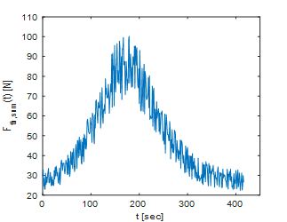
The developed equations were used to simulate the thrust force coefficients, denoted as $K_{t h}=9.61 \times 10^7 \mathrm{Nm}^{-2}$ and $K_{t h, e}=7.68 \times 10^3 \mathrm{Nm}^{-1}$, for a combination of a high-speed steel cutting tool and an aluminum workpiece material in our test setup. The cutting tests were conducted with parameters: a cutting depth $(w)$ of $0.5 \mathrm{~mm}$ and a rotational speed $(\Omega)$ of $280 \mathrm{rpm}$. The aluminum workpiece had a length $(l)$ of $973 \mathrm{~mm}$, a diameter $(D)$ of $20 \mathrm{~mm}$, a measured tensile modulus $(E)$ of $71.3 \mathrm{GPa}$, and a density $(\rho)$ of $2832 \mathrm{~kg} / \mathrm{m}^3$. The feed rate was set at $f=h=0.5 \mathrm{~mm}$ per revolution, resulting in a feed rate (v) of $0.0023 \mathrm{~m} / \mathrm{s}$. The thrust force $\left(F_{t h, s u m}\right)$ was measured by the dynamometer and sampled every second, as depicted in Figure 9. Notably, $F_{t h, s u m}(t)$ was observed to reach a minimum value near the support points, where the tool experiences the least reactive loading from the deformed workpiece. This trend becomes more evident when both the measured and modelled thrust forces are compared on the same graph.
Figure 9. Instantaneous thrust force $F_{th,sum }(t)$ sampled every second for Model 1
Shafts usually pass through holes so the maximum diameter of the machined part should not be more than the minimum diameter of the hole in the tolerance range of the hole if a clearance fit is specified. If an interference fit is specified, the minimum diameter of the machined part should be more than the maximum diameter of the hole in the tolerance range of the hole. If the tolerance of the hole is specified in percentage as $D_H \pm P_H$ then the maximum diameter of the hole $D_{\max }$ must obey.
$D_{\max }<D_H\left(1-\frac{P_H}{100}\right)$ (53)
For a clearance fit while for an interference fit, the relation becomes:
$D_{\min }>D_H\left(1+\frac{P_H}{100}\right)$ (54)
If a transition fit is specified, a pair of conditions that must be satisfied reads:
$D_{\text {min }}<D_H\left(1-\frac{P_H}{100}\right) $ (55)
$D_{\max }<D_H\left(1+\frac{P_H}{100}\right)$ (56)
It is expected that $D_{\min }$ should be equal to $D-2 w$. The maximum value of $D(t)$ should occur at the value of time when:
$\frac{d D(t)}{d t}=0$ (57)
The values of $t$ satisfying these equations are then inserted in (47) and (48) to obtain $D_{\max }$ for both Model 1 and Model 2. A simpler way to estimate $D_{\max }$ is to plot $D(t)$ given in Eq. (47) and Eq. (48) and read $D_{\max }$ from the graph.
In machining, workpiece material extrudes through the shear plane to form chips in much the same way as fluid would flow through a channel. Therefore, material removal rate would have been expected to be deterministically given as:
$\mathrm{MRR}=\rho w h V_t$ (58)
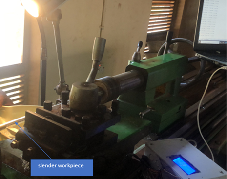
The diameter of the workpiece used in the cutting test is D=15mm. After machining, the diameters of the product along its length and the locations of the diameters were measured with vernier callipers. Then the maximum diameter and the location of the maximum diameter were noted. Also, the minimum diameter and the location of the minimum diameter were noted. Figure 10 shows the setup and the process of the cutting test on the slender workpiece.
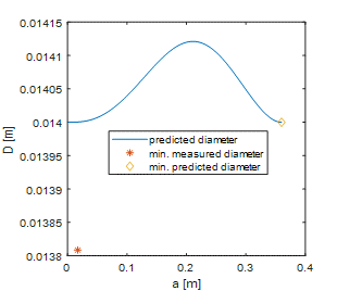
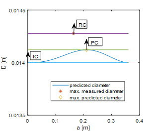
Using Eq. (47), the diameter distribution of the sample is calculated. The results are shown in Figures 11 and 12 for the maximum and minimum diameters. It can be seen that the prediction is relatively correct, see also Table 1 for a comparison of the predicted and measured values. This means that relative to the measured diameter, the prediction can satisfy a clearance fit if the prediction is less that the measured diameter, which is the case. Given the desired diameter of 15-0.5×2=14mm, the clearance fit specification would have meant that the minimum hole diameter should be more than 14mm, but in light of the predicted maximum diameter of 14.1mm, the clearance fit specification can then be adjusted to mean that hole diameter is more than 14.1mm. This adjusted specification is more realistic than the specification that does not consider the effects of flexibility since the real specification that is based on the real (measured) maximum diameter is that hole diameter is more than 14.3mm. This is illustrated in Figure 13 which depicts the minimum hole diameters for the ideal (intended) clearance (IC), predicted clearance (PC) and real clearance (RC).
Since the minimum diameter of the machined part should be more than the maximum diameter of the hole in the tolerance range of the hole for an interference fit, interference fit is satisfied by the prediction relative to the measurement when the former is greater than the latter, which is the case. The values are shown in Table 2.
Figure 10. The setup and the process of the cutting test on the slender workpiece
Figure 11. A predicted diameter distribution and a comparison of the predicted and measured maximum diameter
Figure 12. A predicted diameter distribution and a comparison of the predicted and measured minimum diameter
Table 1. Comparison of measured and predicted maximum diameters of the workpiece
|
Feed Speed v [m/s] |
Feed h [m/rev] |
Predicted Maximum Diameter $D_{\max , p}$ [m] |
Predicted Location of Maximum Diameter $a_{\max , p}$ [m] |
Measured Maximum Diameter $D_{\max , e}$ [m] |
Measured Location of Maximum Diameter $a_{\max , e}$ [m] |
|
0.0023 |
0.0005 |
0.0141 |
0.1640 |
0.0143 |
0.2107 |
Table 2. Comparison of measured and predicted minimum diameters of the workpiece
|
Feed Speed v [m/s] |
Feed h [m/rev] |
Predicted Minimum Diameter $D_{\max , p}$ [m] |
Predicted Location of Minimum Diameter $a_{\max , p}$ [m] |
Measured Minimum Diameter $D_{\max , e}$ [m] |
Measured Location of Minimum Diameter $a_{\max , e}$ [m] |
|
0.0023 |
0.0005 |
0.0140 |
0.3600 |
0.0138 |
0.0170 |
Figure 13. The ideal, predicted, and real minimum hole diameters for clearance fit
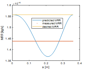
Using the parameters applicable to the test, the MRR is computed using Eq. (42) and the results are shown in Figure 14. As expected, flexibility of the slender workpiece reduced MRR, and the effect is more pronounced the farther from the two ends. The desired MRR is calculated using Eq. (58). Since the desire MRR is fixed at 0.15570g/s, it is plotted as a horizontal line in Figure 14. Therefore, the prediction that considers flexibility gives that flexibility reduces productivity. By weighing the workpiece before and after machining and noting the machining time, the material removal rate was measured to be 0.143g/s and plotted as a fixed line in Figure 14. The measured MRR is comparable to mean of the computed MRR of 0.14685g/s.
Figure 14. Material removal rate
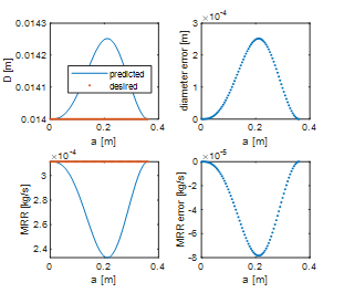
As seen in the preceding section, developed model can adequately capture reality of the effects of flexibility of slender workpieces on form error. Therefore, the model can be used to carry out parametric studies of the machining process. The parameters considered in this section are the cutting process parameters; feed, depth of cut and spindle speed. Comparison of the vertical scales of Figures 15 to 17 shows that increasing the feed increases the deviation of the maximum diameter from the desired diameter thus increasing the chances of not meeting with the tolerance conditions specified on the basis of the desired diameter.
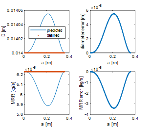
Figure 15. Variation of diameter and MRR at feed of 0.2mm
Figure 16. Variation of diameter and MRR at feed of 1mm
Figure 17. Variation of diameter and MRR at feed of 1.5mm
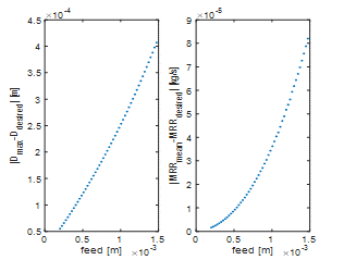
Figure 18. Variation of accuracy and productivity indicators with feed when w=0.5mm and $\Omega$=280rpm
Figure 19. Variation of accuracy and productivity indicators with depth of cut when h=f=0.5mm and Ω=280rpm
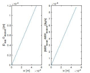
Figure 20. Variation of accuracy and productivity indicators with spindle speed when w=0.5mm and h=f=0.5mm
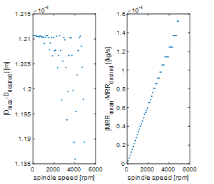
In order to have a very clear picture of how each of the cutting process parameters affect the accuracy and productivity of machining slender workpieces, the appropriate performance criteria are computed on varying each of the cutting process parameters. The performance criterion used for accuracy is the magnitude of the deviation of the maximum of the predicted diameter from the desired diameter while the performance criterion used for productivity is the magnitude of the deviation of the mean of the predicted MRR from the desired MRR. The results are shown in Figures 18 to 20.
The findings showed that as the feed rate, depth of cut, and spindle speed were incrementally raised from 0.5 to 1.5meters, 0 to 6meters, and 0 to 500rpm, respectively, there was an observable increase in the difference between the predicted Material Removal Rate (MRR) and the desired MRR. These differences escalated from 0.1 to 8.2kg/sec, 0 to 8.9kg/sec, and 0 to 1.58kg/sec. This indicates that, under the existing machining conditions and in accordance with the workpiece specifications, productivity can be assured. Moreover, when the feed rate and depth of cut were increased from 0.2 to 1.5meters and 0 to 5meters, the disparities between the predicted and desired diameters also grew, expanding from 0.5 to 4.1meters and 0 to 1.2meters, respectively. However, when the spindle speed was raised from 0 to 500rpm, the deviation exhibited a fluctuating pattern with a gradual reduction over time. This suggests that, at the given machining parameters for feed rate and depth of cut, the accuracy of the machined part can be guaranteed. Nevertheless, with a spindle speed of 350rpm, the accuracy may become uncertain and less reliable. With such plots, specified tolerance ranges could be met by choosing parameter sets that meet the specifications. For example, it can be seen in Figure 20 that it is possible to choose a higher spindle speed that simultaneously reduces form error and improves productivity.
Development of theoretical and numerical framework for selecting the cutting process parameters to enhance the productivity, integrity, and accuracy of turned slender parts is studied. The method involved theoretical modelling that expresses material removal rate and form error in terms of cutting process parameters, workpiece flexibility parameters, workpiece geometrical parameters, and kinematic parameters. Cutting tests were carried out in validation of the arising theoretical and numerical results. Parametric studies were carried out using the developed computational model to understand the trend of accuracy and productivity with variation of cutting process parameter. An illustration is that clearance fit that should have been based on a minimum hole diameter of 14mm is adjusted to a hole diameter of 14.1mm due the modelled flexibility effects. The unneeded form error induced by flexibility can be captured correctly enough computationally. Comparison of the vertical scales of Figures 16 to 18 shows that increasing the feed increases the deviation of the maximum diameter from the desired diameter thus increasing the chances of not meeting with the tolerance conditions specified on the basis of the desired diameter. As expected, the parametric study shows that flexibility of the slender workpiece reduced MRR. The results showed that deviation of predicted values of MRR from the desired values rises with rise of the cutting process parameters; feed, depth of cut and spindle speed. The results also showed that deviation of predicted diameter from the desired values rises with rise of feed and depth of cut but has fluctuating and slowly falling trend with the rise of spindle speed. Based on the results of the parametric studies, specified tolerance ranges could be met by choosing parameter sets that meet the specifications. The framework may not adequately address the tolerances required for specific applications, potentially leading to deviations from desired part dimensions. Overcoming these limitations often involves continuous research and development efforts, incorporating real-world data, and improving the accuracy and adaptability of the framework for specific machining scenarios. The parametric study results can be used as a framework for the selection of cutting process parameter to enhance the productivity, integrity, and accuracy of turned slender parts.
The authors appreciate the managements of Afe Babalola University for paying the article processing charges and The Bells University of Technology for providing conducive environment for researchers to thrive.
|
Tct |
complete machine adjusting time, s |
|
Ti |
controlling or inactive time, s |
|
Tc |
real machining time, s |
|
TCT |
time needed for a single changing, s |
|
Tm |
total time for machining, s |
|
Lc |
complete cut length, mm |
|
s |
rate of feed, mm.rev-1 |
|
Ω |
spindle speed, rpm |
|
Vc |
speed of cu of cut, m.s-2 |
|
D |
diameter of job, mm |
|
TL |
taylor’s tool life |
|
Fc |
tangential cutting force component, N |
|
Nc |
feed cutting force component, N |
|
Fth |
thrust cutting force component, N |
|
Fsp |
shear force component on the shear plane |
|
Nsp |
normal force component on the shear plane |
|
Frf |
frictional force component of the rake face |
|
Nrf |
normal force component of the rake face |
|
rch |
chip thickness ratio |
|
h |
undeformed chip thickness (mm) |
|
hch |
chip thickness, mm |
|
Vch |
chip velocity on the rake face, m.s-2 |
|
Vt |
tangential velocity, m.s-2 |
|
w |
depth of cut, mm |
|
$\sigma_{\mathrm{sp}}$ |
yield normal stress of the material, N.mm-2 |
|
$\tau_{s p}$ |
yield shear stress of the material, N.mm-2 |
|
Kf |
feed cutting force coefficient, N.mm-2 |
|
Kt |
tangential cutting force coefficient, N.mm-2 |
|
Kth |
thrust cutting force coefficient, N.mm-2 |
|
Kf, e |
Feed edge force coefficient, N.mm-1 |
|
Kt, e |
Tangential edge force coefficient, N.mm-1 |
|
Kth, e |
thrust edge force coefficient, N.mm-1 |
|
E |
young’s modulus, N.mm-2 |
|
I |
moment of inertia, mm-4 |
|
l |
length of the workpiece, mm |
|
y |
beam deflection, mm |
|
F |
the applied load on the beam, N |
|
M1 |
bending moment at point A, Nm |
|
MAB |
bending moment at point AB, Nm |
|
MBC |
bending moment at point BC, Nm |
|
yAB |
deflection along AB, mm |
|
YBC |
deflection along BC, mm |
|
R1 |
reaction at support A, N |
|
R2 |
reaction at support C, N |
|
$\rho$ |
density of the workpiece, kg.m-3 |
|
x |
distance from point A to the point of interest along the length of the workpiece, mm |
|
w(a) |
actual depth of cut, mm |
|
a |
distance of the load from fixed end A, mm |
|
b |
distance of the load from end C, mm |
|
ϑ |
non-zero approach angle, deg. |
|
w(t) |
instantaneous depth of cut, mm |
|
MRR |
material removal rate, kg.m-3 |
|
Dmax |
maximum diameter of the workpiece, mm |
|
$\bar{D}$ |
average diameter of the workpiece, mm |
|
m |
total amount of material removed, kg |
|
t |
time, s |
|
y(t) |
instantaneous deflection, mm |
|
yi |
predicted values |
|
Ti |
experimental values |
|
R2 |
coefficient of determination |
|
RMSE |
root mean square error |
|
MBE |
mean biased error |
|
MABE |
mean absolute biased error |
|
MPA |
mean percentage error |
|
Greek symbols |
|
|
$\alpha$ |
rake angel, deg |
|
$\beta$ |
friction angle, deg |
|
$\varphi$ |
shear angle, deg |
[1] Lu, K.B., Lian, Z.S., Gu, F.S., Liu, H.J. (2018). Model-based chatter stability prediction and detection for the turning of a flexible workpiece. Mechanical Systems and Signal Processing, 100: 814-826. https://doi.org/10.1016/j.ymssp.2017.08.022
[2] Kiran, K., Kayacan, M.C. (2019). Effect of material removal on workpiece dynamics in milling: Modeling and measurement. Precision Engineering, 60: 506-519. https://doi.org/10.1016/j.precisioneng.2019.09.003
[3] Katz, R., Lee, C.W., Ulsoy, A.G., Scott, R.A. (1989). Turning of slender workpieces: Modeling and experiments. Mechanical Systems and Signal Processing, 3(2): 195-205. https://doi.org/10.1016/0888-3270(89)90016-2
[4] Petrakov, Y., Danylchenko, M., Petryshyn, A. (2019). Prediction of chatter stability in turning. Eastern-European Journal of Enterprise Technologies, 5(1): 58-64. https://doi.org/10.15587/1729-4061.2019.177291
[5] Nicolescu, C.M. (1996). On-line identification and control of dynamic characteristics of slender workpieces in turning. Journal of Materials Processing Technology, 58(4): 374-378. https://doi.org/10.1016/0924-0136(95)02210-4
[6] Osueke, C.O., Ezugwu, C.A.K., Adeoye, A.O.M. (2015). Dynamic approach to optimization of material removal rate through programmed optimal choice of milling process parameters, part 1: Validation of result with CNC simulation. International Journal of innovative research in Advanced Engineering, 2(5): 118-129.
[7] Yue, H.T., Guo, C.G., Li, Q., Zhao, L.J., Hao, G.B. (2020). Thermal error modeling of CNC milling machining spindle based on an adaptive chaos particle swarm optimization algorithm. Journal of the Brazilian Society of Mechanical Sciences and Engineering, 42: 1-13. https://doi.org/10.1007/s40430-020-02514-z
[8] Ramesh, R., Mannan, M.A., Poo, A.N. (2000). Error compensation in machine tools-a review: Part I: Geometric, cutting-force induced and fixture-dependent errors. International Journal of Machine Tools and Manufacture, 40(9): 1235-1256. https://doi.org/10.1016/S0890-6955(00)00009-2
[9] Lu, K.B., Jing, M.Q., Zhang, X.L., Dong, G.H., Liu, H. (2015). An effective optimization algorithm for multipass turning of flexible workpieces. Journal of Intelligent Manufacturing, 26: 831-840. https://doi.org/10.1007/s10845-013-0838-7
[10] Lu, K.B., Zhang, Z.D., Jing, M.Q., Wang, Y.L., Liu, H., Wu, T.H. (2016). Dynamic optimization of multipass turning of a flexible workpiece considering the effect of cutting sequence. The International Journal of Advanced Manufacturing Technology, 85: 325-335. https://doi.org/10.1007/s00170-015-7902-8
[11] Chen, Z., Peng, R.L., Zhou, J.M., M’Saoubi, R., Gustafsson, D., Moverare, J. (2019). Effect of machining parameters on cutting force and surface integrity when high-speed turning AD 730™ with PCBN tools. The International Journal of Advanced Manufacturing Technology, 100: 2601-2615. https://doi.org/10.1007/s00170-018-2792-1
[12] Abhilash, P.M., Chakradhar, D. (2020). Surface integrity comparison of wire electric discharge machined inconel 718 surfaces at different machining stabilities. Procedia CIRP, 87: 228-233. https://doi.org/10.1016/j.procir.2020.02.037
[13] Spescha, D., Weikert, S., Wegener, K. (2020). Simulation in the design of machine tools. Reinventing Mechatronics: Developing Future Directions for Mechatronics. https://doi.org/10.1007/978-3-030-29131-0_11
[14] Fischer, A., Eberhard, P. (2011). Simulation-based stability analysis of a thin-walled cylinder during turning with improvements using an adaptronic turning chisel. Archive of Mechanical Engineering, 58(4): 367-391. https://doi.org/10.2478/v10180-011-0023-5
[15] Sun, T., Qin, L.F., Fu, Y.C., Hou, J.M. (2019). Chatter stability of orthogonal turn-milling analyzed by complete discretization method. Precision Engineering, 56: 87-95. https://doi.org/10.1016/j.precisioneng.2018.10.012
[16] Zhao, G.J., Jiang, S.C., Dong, K., Xu, Q.W., Zhang, Z.L., Lu, L. (2022). Influence analysis of geometric error and compensation method for four-axis machining tools with two rotary axes. Machines, 10(7): 586. https://doi.org/10.3390/machines10070586
[17] Woźniak, M., Parus, A. (2019). Active vibration control of a slender workpiece during turning. Journal of Machine Construction and Maintenance-Problemy Eksploatacji, 112: 17-23.
[18] Beri, B., Meszaros, G., Stepan, G. (2021). Machining of slender workpieces subjected to time-periodic axial force: Stability and chatter suppression. Journal of Sound and Vibration, 504: 116114. https://doi.org/10.1016/j.jsv.2021.116114
[19] Sekar, M., Srinivas, J., Kotaiah, K.R., Yang, S.H. (2009). Stability analysis of turning process with tailstock-supported workpiece. The International Journal of Advanced Manufacturing Technology, 43: 862-871. https://doi.org/10.1007/s00170-008-1764-2
[20] Gururaja, S., Singh, K.K., Mittal, R.K. (2022). Analysis of numerical method for modal analysis of thin-walled structures for achieving low-cost manufacturing. In North-East Research Conclave, Singapore: Springer Nature Singapore, 1-20. https://doi.org/10.1007/978-981-19-8452-5_1
[21] Urbikain, G., De Lacalle, L.L., Campa, F.J., Fernández, A., Elías, A. (2012). Stability prediction in straight turning of a flexible workpiece by collocation method. International Journal of Machine Tools and Manufacture, 54: 73-81. https://doi.org/10.1016/j.ijmachtools.2011.11.008
[22] Guo, P., Li, Z., Xiong, Z.W., Zhang, S.J. (2023). A theoretical and experimental investigation into tool setting induced form error in diamond turning of micro-lens array. The International Journal of Advanced Manufacturing Technology, 124(7-8): 2515-2525. https://doi.org/10.1007/s00170-022-10643-z
[23] Yu, D.P., Hong, G.S., San Wong, Y. (2012). Profile error compensation in fast tool servo diamond turning of micro-structured surfaces. International Journal of Machine Tools and Manufacture, 52(1): 13-23. https://doi.org/10.1016/j.ijmachtools.2011.08.010
[24] Liu, X.L., Zhang, X.D., Fang, F.Z., Liu, S.G. (2016). Identification and compensation of main machining errors on surface form accuracy in ultra-precision diamond turning. International Journal of Machine Tools and Manufacture, 105: 45-57. https://doi.org/10.1016/j.ijmachtools.2016.03.001
[25] Wang, B., Liu, Z.Q., Cai, Y.K., Luo, X.C., Ma, H.F., Song, Q.H., Xiong, Z.H. (2021). Advancements in material removal mechanism and surface integrity of high speed metal cutting: A review. International Journal of Machine Tools and Manufacture, 166: 103744. https://doi.org/10.1016/j.ijmachtools.2021.103744
[26] Xiao, X.S., Yu, Q.H., Chen, G.L., Liang, R.G. (2020). Locating optimal freeform surfaces for off-axis optical systems. Optics Communications, 467: 125757. https://doi.org/10.1016/j.optcom.2020.125757
[27] Misaka, T., Herwan, J., Ryabov, O., Kano, S., Sawada, H., Kasashima, N., Furukawa, Y. (2020). Prediction of surface roughness in CNC turning by model-assisted response surface method. Precision Engineering, 62: 196-203. https://doi.org/10.1016/j.precisioneng.2019.12.004
[28] Ozoegwu, C., Ofochebe, S., Ezugwu, C. (2016). Time minimization of pocketing by zigzag passes along stability limit. The International Journal of Advanced Manufacturing Technology, 86: 581-601. https://doi.org/10.1007/s00170-015-8108-9
[29] Okonkwo, U.C., Osueke, C.O., Ezugwu, C.A.K. (2015). Minimizing machining time in pocket milling based on optimal combination of the three basic prescription 1 parameters. International Research Journal of Innovative Engineering, 1(4): 12-34.
[30] Ozoegwu, C., Ezugwu, C. (2015). Minimizing pocketing time by selecting most optimized chronology of tool passes. The International Journal of Advanced Manufacturing Technology, 81: 1667-1682. https://doi.org/10.1007/s00170-015-6943-3
[31] Song, L.Q., Zhao, X.S., Zhang, Q., Shi, D.Q., Sun, T. (2023). A geometric error measurement method for five-axis ultra-precision machine tools. The International Journal of Advanced Manufacturing Technology, 126(3-4): 1379-1395. https://doi.org/10.1007/s00170-023-11181-y
[32] Nagayama, K., Yan, J.W. (2021). Deterministic error compensation for slow tool servo-driven diamond turning of freeform surface with nanometric form accuracy. Journal of Manufacturing Processes, 64: 45-57. https://doi.org/10.1016/j.jmapro.2021.01.015
[33] Gao, W., Haitjema, H., Fang, F.Z., Leach, R.K., Cheung, C.F., Savio, E., Linares, J.M. (2019). On-machine and in-process surface metrology for precision manufacturing. CIRP Annals, 68(2): 843-866. https://doi.org/10.1016/j.cirp.2019.05.005
[34] Okonkwo, U.C., Okokpujie, I.P., Sinebe, J.E., Ezugwu, C.A.K. (2015). Comparative analysis of aluminium surface roughness in end-milling under dry and minimum quantity lubrication (MQL) conditions. Manufacturing Review, 2: 30. https://doi.org/10.1051/mfreview/2015033
[35] Ezugwu, C.A., Osueke, C.O., Onokwai, A.O., Uguru-Okorie, D.C., Ikpotokin, I., Ibikunle, R.A. (2018). Modeling of regenerative chatter of a milling process to delineate stable cutting region from unstable region. International Journal of Mechanical Engineering and Technology, 9(11): 748-757.
[36] Ezugwu, C.A.K., Okonkwo, U.C., Sinebe, J.E., Okokpujie, I.P. (2016). Stability analysis of model regenerative chatter of milling process using first order least square full discretization method. International Journal of Mechanics and Applications, 6(3): 49-62. https://doi.org/10.5923/j.mechanics.20160603.03
[37] Li, Z.L., Tuysuz, O., Zhu, L.M., Altintas, Y. (2018). Surface form error prediction in five-axis flank milling of thin-walled parts. International Journal of Machine Tools and Manufacture, 128: 21-32. https://doi.org/10.1016/j.ijmachtools.2018.01.005
[38] Tong, Z., Zhong, W.B., To, S., Zeng, W.H. (2020). Fast-tool-servo micro-grooving freeform surfaces with embedded metrology. CIRP Annals, 69(1): 505-508. https://doi.org/10.1016/j.cirp.2020.04.111
[39] Hu, Q., Chen, Y.P., Yang, J.X. (2020). On-line contour error estimation and control for corner smoothed five-axis tool paths. International Journal of Mechanical Sciences, 171: 105377. https://doi.org/10.1016/j.ijmecsci.2019.105377
[40] Yang, J.X., Ai, W., Liu, Y.X., Chen, B. (2018). Kinematics model and trajectory interpolation algorithm for CNC turning of non-circular profiles. Precision Engineering, 54: 212-221. https://doi.org/10.1016/j.precisioneng.2018.05.014
[41] Ezugwu, C.A.K., Fayomi, O.S.I., Onifade, M.K., Adeoye, A.O.M., Okokpujie, I.P. (2023). Modelling the effects of workpiece flexibility on cutting performance in turning operations. Journal Européen des Systèmes Automatisés, 56(4): 615-625. https://doi.org/10.18280/jesa.560411
[42] Qehaja, N., Jakupi, K., Bunjaku, A., Bruçi, M., Osmani, H. (2015). Effect of machining parameters and machining time on surface roughness in dry turning process. Procedia Engineering, 100: 135-140. https://doi.org/10.1016/j.proeng.2015.01.351
[43] Cianetti, F., Morettini, G., Palmieri, M., Zucca, G. (2019). Virtual qualification of aircraft parts: Test simulation or acceptable evidence? Procedia Structural Integrity, 24: 526-540. https://doi.org/10.1016/j.prostr.2020.02.047
[44] Nisbett, J.K., Budynas, R.G. (2002). Shigley’s Mechanical Engineering Design, Ninth edition. Mechanical Engineering.
[45] Hanif, M.I., Aamir, M., Ahmed, N., Maqsood, S., Muhammad, R., Akhtar, R., Hussain, I. (2019). Optimization of facing process by indigenously developed force dynamometer. The International Journal of Advanced Manufacturing Technology, 100: 1893-1905. https://doi.org/10.1007/s00170-018-2829-5