Dhiyaa Sheltag Shanan![]() | Saleem Khalefa Kadhim*
| Saleem Khalefa Kadhim*![]()
© 2023 IIETA. This article is published by IIETA and is licensed under the CC BY 4.0 license (http://creativecommons.org/licenses/by/4.0/).
OPEN ACCESS
Ventilator designs, pivotal in providing respiratory support to patients, often grapple with performance optimization challenges due to variable patient conditions and intricate mechanical components. This research strives to identify the optimal control strategy that can assure maximal patient safety and efficient ventilator operation. We compared three control strategies: the conventional Proportional-Integral-Derivative (PID) control, the Nonlinear PID control, and the sliding mode control (SMC) equipped with signum function triggers. Our studies underscored the preeminence of SMC in controlling airway pressure, exhibiting a rapid and disturbance-free response. However, while SMC ensured smooth patient airflow in flow rate control, it exhibited a slightly delayed response. The research thus posits SMC as a promising contender, particularly in light of the sophisticated design requirements of contemporary ventilators. Through this investigation, we aim to offer a robust control solution capable of enhancing current ventilator operations to ensure superior patient safety and efficiency.
ventilator, PID control, nonlinear PID control, sliding mode control
Ventilators are pivotal medical devices used to provide respiratory support to patients in dire need, especially those with respiratory issues. Despite the existing extensive research on the design and control of ventilators aimed at ensuring patient safety and optimizing performance, there exists a significant gap in understanding the best control strategies.
Several preceding research studies have investigated a wide range of control strategies, thereby elucidating the crucial outcomes and shortcomings observed in prior studies within this field, as outlined in the Martin et al. [1] investigated the impact of different ventilation modes on patient outcomes. They found that a synchronized intermittent mandatory ventilation mode resulted in improved patient comfort but had limitations in providing optimal ventilation for certain patient populations.
Rinkeviciene and Kriaucinas [2] proposed a closed-loop control system for ventilators using fuzzy logic control (FLC). Their findings demonstrated improved patient-ventilator synchronization, but the complexity of the FL controller posed challenges in implementation and tuning. Ingaramo et al. [3] examined the effects of positive end-expiratory pressure (PEEP) on lung recruitment and oxygenation. They observed that higher PEEP levels improved oxygenation but could lead to over distension of the lungs in certain cases. Walter and Leonhardt [4] have categorized various automatic control levels in artificial ventilation into three distinct groups based on the degree of interaction between patients and medical devices. Class 1, termed as device-internal control loops, and Class 2, known as patient-oriented control loops, both use control signals measured within the device. The key distinction is that Class 2 allows for patient-device interaction, whereas Class 1 does not. Contrarily, Class 3, named physiological compensatory control loops, employs physiological parameters as its control variable. This study introduces a pressure-based ventilation controller from the Class 2 group, aiming to maintain a consistent target airway pressure.
In the study [5], the PID controller is a widely-used tool in mechanical ventilation. Its adoption can be traced back to the advent of microprocessors. However, the PID controller is often critiqued for its suboptimal performance in systems with variable dynamics, a scenario evident in mechanical ventilation. Variability arises because lung compliance and resistance differ among patients and change in response to lung volumes. To enhance the efficiency of the PID controller in this context, numerous researchers have introduced modifications. These enhancements include integrating an adaptive mechanism [6], implementing optimization strategies [7], and automating the tuning of PID gains [8].
From review of the literature, various controllers have been applied to mechanical ventilation. These include model predictive control [9], variable-gain control [10], and repetitive control [11].
The literature presents nonlinear control approaches that don't necessitate a precise understanding of system dynamics [12, 13]. Notably, SMC stands out as a robust technique adept at managing intricate dynamical systems [14, 15]. The SMC is frequently employed in systems where nominal models and disturbances with known upper bounds exist [16, 17]. It is recognized for its robustness in the face of parameter uncertainties. Yet, traditional SMC controllers can induce high-frequency chattering in excitation signals, restricting their practical use [18]. Beyond the conventional SMCs, intelligent controls like FLC have also been documented and applied in mechanical ventilators [19, 20]. Their study showed improved tracking performance and disturbance rejection but acknowledged the challenge of accurately estimating disturbances in real-time.
Research Gap: Despite the extensive work, gaps persist, particularly concerning real-time implementation, computational complexity, and system interpretability of the controller strategies. Further, a comprehensive comparison and assessment of the various control strategies is lacking.
Objective: This study seeks to address these gaps by proposing robust control strategies for ventilators and offering a thorough comparison and evaluation of different control methods. Specifically, we aim to scrutinize the effectiveness of conventional PID control, nonlinear PID control, and SMC with two signum functions serving as triggers for control actions. Through our research, we aspire to advance ventilator technology, ensuring patient safety and optimal ventilator performance.
The mathematical modeling of a ventilator system is the foundation upon which different control strategies, as implied by our paper's title, are built and evaluated. This section lays down the fundamental groundwork for understanding the system dynamics, which will be instrumental when comparing various control approaches in subsequent sections.
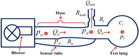
Figure 1 illustrates the respiratory system, indicating various pressures in red, flows in blue, resistances, and compliance. The mechanical ventilation device comprises a blower unit powered electrically, creating the necessary pressure (Po) for the patient's lungs through the hose medium covering. Mathematical models, as shown in various studies [21, 22], have been pivotal in addressing complex engineering challenges, especially in elucidating patient lung mechanics and enhancing ventilation therapies [23].
Figure 1. Schematic of a mechanical ventilation unit
Assumptions: For the purpose of this study, it's assumed that standard resistances of the hose, leak channel, and patient's lungs are known. This is a commonly accepted assumption in several studies within this domain [24-26]. By assuming this, it simplifies the modeling process and allows for a focused analysis of control strategies. However, it's important to note that any deviations from these standard resistances in real-life scenarios might lead to variations in the system behavior, which could necessitate adaptive or robust control techniques to manage.
The lungs draw in air via an airflow rate (Qo), while simultaneously releasing a flow rate of (Qleak) through a leaky hose, leaving (Qp) as the remaining exhaled airflow [25].
$\mathrm{Q_{\text {p}}}=\mathrm{Q_{\text {o}}}-\mathrm{Q_{\text {leak }}}$ (1)
The flow of air from the blower to the lung is like the flow of current inside an electric wire, wherefore the pressure is more like the electric voltage, and the system may be viewed as an electric circuit in which resistances are depicted by everything that obstructs the air, or a potential difference represented by pressures and the current represented by the flow. Therefore, the patient air flow shown in the Figure 1 can be expressed by the following equation according to Ohm's law [26]. Inside the module, a pressure sensor gauges the airway pressure, denoted as Pa.
The aim of the control system is to track the measured pressure and make sure that it corresponds to the desired set point, Pr. As a result, the error equation is formulated as follows [24]:
$\mathrm{e}=\mathrm{P}_{\mathrm{r}}-\mathrm{P}_{\mathrm{a}}$ (2)
Assuming that the standard resistances of the hose, leak channel, and patient lungs have been identified, will be express the flow rates of the blower, patient, and leak as functions of these resistances, as shown below [24-26]:
$\mathrm{Q}_{\mathrm{o}}=\frac{\mathrm{P}_{\mathrm{o}}-\mathrm{P}_{\mathrm{a}}}{\mathrm{R}_{\mathrm{h}}}$ (3)
$\mathrm{Q}_{\text {leak }}=\frac{\mathrm{P}_{\mathrm{a}}}{\mathrm{R}_{\text {leak }}}$ (4)
$\mathrm{Q}_{\mathrm{p}}=\frac{\mathrm{P}_{\mathrm{a}}-\mathrm{P}_{\text {lung }}}{\mathrm{R}_{\text {lung }}}$ (5)
Lungs pressure Plung dynamics are satisfies the following differential equation:
$\mathrm{P_{\text {lung }}}=\frac{1}{\mathrm{c_{\text {lung }}}} \cdot \mathrm{Q_p}$ (6)
In Eq. (5), Plung can be likened to voltage, and Qp can be compared to current. When Eqs. (5) and (6) are merged, the resulting expression is as follows:
$\mathrm{P}_{\text {lung }}=\frac{\mathrm{P}_{\mathrm{a}}-\mathrm{P}_{\text {lung }}}{\mathrm{C}_{\text {lung }} \cdot \mathrm{R}_{\text {lung }}}$ (7)
To obtain airway pressure Pa, Formulate the equation for airway pressure, Pa, using substitution of Eqs. (3), (4) and (5) in Eq. (1).
$\frac{\mathrm{P}_{\mathrm{a}}-\mathrm{P}_{\text {lung }}}{\mathrm{R}_{\text {lung }}}=\frac{\mathrm{P}_{\mathrm{o}}-\mathrm{P}_{\mathrm{a}}}{\mathrm{R}_{\mathrm{h}}}-\frac{\mathrm{P}_{\mathrm{a}}}{\mathrm{R}_{\text {leak }}}$ (8)
$\frac{\mathrm{P}_{\mathrm{a}}}{\mathrm{R}_{\text {lung }}}-\frac{\mathrm{P}_{\text {lung }}}{\mathrm{R}_{\text {lung }}}=\frac{\mathrm{P}_{\mathrm{o}}}{\mathrm{R}_{\mathrm{h}}}-\frac{\mathrm{P}_{\mathrm{a}}}{\mathrm{R}_{\mathrm{h}}}-\frac{\mathrm{P}_{\mathrm{a}}}{\mathrm{R}_{\text {leak }}}$ (9)
$\frac{\mathrm{P}_{\mathrm{a}}}{\mathrm{R}_{\text {lung }}}+\frac{\mathrm{P}_{\mathrm{a}}}{\mathrm{R}_{\mathrm{h}}}+\frac{\mathrm{P}_{\mathrm{a}}}{\mathrm{R}_{\text {leak }}}=\frac{\mathrm{P}_{\mathrm{o}}}{\mathrm{R}_{\mathrm{h}}}+\frac{\mathrm{P}_{\text {lung }}}{\mathrm{R}_{\text {lung }}}$ (10)
$\mathrm{P}_{\mathrm{a}}\left(\frac{1}{\mathrm{R}_{\text {lung }}}+\frac{1}{\mathrm{R}_{\mathrm{h}}}+\frac{1}{\mathrm{R}_{\text {leak }}}\right)=\frac{\mathrm{P}_{\mathrm{o}}}{\mathrm{R}_{\mathrm{h}}}+\frac{\mathrm{P}_{\text {lung }}}{\mathrm{R}_{\text {lung }}}$ (11)
$\mathrm{P}_{\mathrm{a}}=\frac{\frac{1}{\mathrm{R}_{\mathrm{h}}} \cdot \mathrm{P}_{\mathrm{o}}+\frac{1}{\mathrm{R}_{\text {lung }}} \cdot \mathrm{P}_{\text {lung }}}{\frac{1}{\mathrm{R}_{\text {lung }}}+\frac{1}{\mathrm{R}_{\mathrm{h}}}+\frac{1}{\mathrm{R}_{\text {leak }}}}$ (12)
Substituting the airway pressure expression in Eq. (12) into the differential equation for lung dynamics in Eq. (7) results in the following revised equation:
$\mathrm{P}_{\text {lung }}=\frac{-\mathrm{P}_{\text {lung }}\left(\frac{1}{\mathrm{R}_{\mathrm{h}}}+\frac{1}{\mathrm{R}_{\text {leak }}}\right)+\frac{1}{\mathrm{R}_{\mathrm{h}}} \cdot \mathrm{P}_{\mathrm{o}}}{\mathrm{C}_{\text {lung }} \cdot \mathrm{R}_{\text {lung }}\left(\frac{1}{\mathrm{R}_{\text {lung }}}+\frac{1}{\mathrm{R}_{\mathrm{h}}}+\frac{1}{\mathrm{R}_{\text {leak }}}\right)}$ (13)
Given Eqs. (5), (12), and (13). The system consisting of the patient and hose can be expressed as a linear state-space system, with Po serving as the input, out put $\left[\begin{array}{c}\mathrm{P}_{\mathrm{a}} \\ \mathrm{Q}_{\mathrm{p}}\end{array}\right]$, and the state Plung.
$\mathrm{P}_{\text {lung }}=\mathrm{A_h} \mathrm{P}_{\text {lung }}+\mathrm{B_h} \mathrm{P_o}$ (14)
$\left[\begin{array}{l}\mathrm{P}_{\mathrm{a}} \\ \mathrm{Q}_{\mathrm{p}}\end{array}\right]=\mathrm{C}_{\mathrm{h}} \mathrm{P}_{\text {lung }}+\mathrm{D}_{\mathrm{h}} \mathrm{P}_{\mathrm{o}}$ (15)
where,
$\mathrm{A_h}=-\frac{\frac{1}{R_h}+\frac{1}{R_{\text {leak }}}}{\mathrm{C}_{\text {lung }} \cdot \mathrm{R}_{\text {lung }}\left(\frac{1}{\mathrm{R}_{\text {lung }}}+\frac{1}{\mathrm{R_h}}+\frac{1}{\mathrm{R}_{\text {leak }}}\right)}$ (16)
$\mathrm{B}_{\mathrm{h}}=\frac{\frac{1}{\mathrm{R}_{\mathrm{h}}}}{\mathrm{C}_{\text {lung }} \cdot \mathrm{R}_{\text {lung }}\left(\frac{1}{\mathrm{R}_{\text {lung }}}+\frac{1}{\mathrm{R}_{\mathrm{h}}}+\frac{1}{\mathrm{R}_{\text {leak }}}\right)}$ (17)
$\mathrm{C}_{\mathrm{h}}=\left[\begin{array}{c}\frac{\frac{1}{\mathrm{R}_{\text {lung }}}}{\frac{1}{\mathrm{R}_{\text {lung }}}+\frac{1}{\mathrm{R}_{\mathrm{h}}}+\frac{1}{\mathrm{R}_{\text {leak }}}} \\ -\frac{\frac{1}{\mathrm{R}_{\mathrm{h}}}+\frac{1}{\mathrm{R}_{\text {leak }}}}{\mathrm{R}_{\text {lung }}\left(\frac{1}{\mathrm{R}_{\text {lung }}}+\frac{1}{\mathrm{R}_{\mathrm{h}}}+\frac{1}{\mathrm{R}_{\text {leak }}}\right)}\end{array}\right]$ (18)
$\mathrm{D}_{\mathrm{h}}=\left[\begin{array}{c}\frac{\frac{1}{\mathrm{R}_{\mathrm{h}}}}{\frac{1}{\mathrm{R}_{\text {lung }}}+\frac{1}{\mathrm{R}_{\mathrm{h}}}+\frac{1}{\mathrm{R}_{\text {leak }}}} \\ \frac{\frac{1}{\mathrm{R}_{\mathrm{h}}}}{\mathrm{R}_{\text {lung }}\left(\frac{1}{\mathrm{R}_{\text {lung }}}+\frac{1}{\mathrm{R}_{\mathrm{h}}}+\frac{1}{\mathrm{R}_{\text {leak }}}\right)}\end{array}\right]$ (19)
Alternatively, this can be represented in transfer function notation as well:
$\mathrm{H}(\mathrm{s})=\mathrm{C}_{\mathrm{h}} \frac{1}{\left(\mathrm{SI}-\mathrm{A}_{\mathrm{h}}\right)} \mathrm{B}_{\mathrm{h}}+\mathrm{D}_{\mathrm{h}}$ (20)
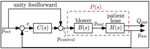
Blower system can effectively produce the desired module output pressure, Po. The blower's qualities have been established based on a steady-state feature that perfectly maps the output pressure target, Pcontrol(s), to the actual output pressure, Po, resulting in a value of 1, as shown in Figure 2. Nevertheless, the blower constitutes a dynamic system with inertia, implying that the actual system experiences roll-off at high frequencies, much like a servo system. A servo system, which employs negative feedback mechanisms, is an electromagnetic apparatus that utilizes electricity to achieve precisely controlled motion [27].
Figure 2, a system in which the closed-loop transfer function has two poles is referred to as a second-order system, though certain second-order systems may have one or two zeros as well, as shown in Figure 2 [27].
Therefore, a control system response must be obtained illustrate the response of a standard second-order system to a step input, a ramp input, and an impulse input. Further, it will be considered the blower can be viewed as an instance of a second-order system, similar to a servo system.
Figure 2. Linear controller is employed in a closed-loop control system C(s)
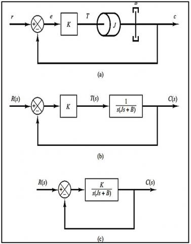
Figure 3a depicts a servo system that comprises load elements, such as inertia and viscous-friction components, as well as a proportional controller. Assume that the control of the output position, c, corresponds to the input position, r. The equation governing the load elements is as follows:
$\mathrm{J} \ddot{\mathrm{c}}+\mathrm{B} \dot{\mathrm{c}}=\mathrm{T}$ (21)
where, T is the torque produced by the proportional controller whose gain is K. J represents the matrix mass moment of inertia, B is the coefficient of viscosity. Assuming zero initial conditions, by obtain the Laplace transforms of both sides of Eq. (21) by applying Laplace transform, Eq. (22) will be obtained:
$\mathrm{Js}^2 \mathrm{C}(\mathrm{s})+\mathrm{BsC}(\mathrm{s})=\mathrm{T}(\mathrm{s})$ (22)
Also, the transfer function linking C(s) and T(s) is given by:
$\frac{\mathrm{C}(s)}{\mathrm{T}(\mathrm{s})}=\frac{1}{s (\mathrm{J} s+\mathrm{B})}$ (23)
Transfer function illustrated in Figure 3a can be redrawn as shown in Figure 3b utilizing this transfer function, which can then be altered to that seen in Figure 3c. The closed-loop transfer function can then be derived as follows:
$\frac{\mathrm{C} (\mathrm{s})}{\mathrm{R} (\mathrm{s})}=\frac{\mathrm{K}}{\mathrm{J} \mathrm{S}^2+\mathrm{B} s+\mathrm{K}}=\frac{\mathrm{K} / \mathrm{J}}{\mathrm{s}^2+(\mathrm{B} / \mathrm{J}) \mathrm{s}+(\mathrm{K} / \mathrm{J})}$ (24)
Figure 3. Servo system in (a); its block diagram in (b); and the simplified block diagram in (c) [27]
The step response of a second-order system can be obtained from the closed-loop transfer function of the system illustrated in Figure 3c, which is given below:
$\frac{\mathrm{C} (\mathrm{s})}{\mathrm{R} (\mathrm{s})}=\frac{\mathrm{K}}{\mathrm{J} \mathrm{S}^2+\mathrm{B} s+\mathrm{K}}$ (25)
This can be expressed in a different form as follows:
$\frac{C (s)}{R (s)}=\frac{K / J}{\left[s+\frac{B}{2 J}+\sqrt{\left(\frac{B}{2 J}\right)^2-\frac{K}{J}}\right]\left[s+\frac{B}{2 J}-\sqrt{\left(\frac{B}{2 J}\right)^2-\frac{K}{J}}\right]}$ (26)
In transient-response analysis, it is more convenient to express the closed-loop poles as follows: B2-4JK<0, the closed-loop poles are complex conjugates, while if B2-4JK≥0, they are real. In the transient-response analysis, it is convenient to write:
$\frac{\mathrm{K}}{\mathrm{J}}=\omega_{\mathrm{n}}^2, \frac{\mathrm{B}}{\mathrm{J}}=2 \zeta \omega_{\mathrm{n}}=2 \sigma$ (27)
where, σ is referred to as the attenuation; ωn, the Undamped natural frequency; and ζ, the damping ratio of the system. The damping ratio ζ is the ratio of the actual damping B to the critical damping or:
$\zeta=\frac{\mathrm{B}}{\mathrm{B}_{\mathrm{c}}}=\frac{\mathrm{B}}{2 \sqrt{\mathrm{JK}}}$ (28)
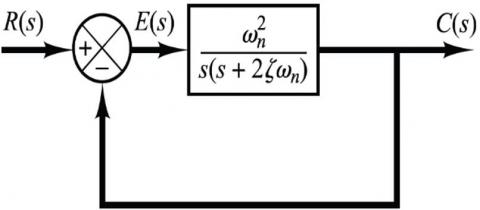
Closed-loop transfer function of the system illustrated in Figure 3c can be expressed in terms of and ωn and then transformed into the form shown in Figure 4. The resulting transfer function for C(s)/R(s) is given by Eq. (24) can be written:
$\frac{\mathrm{C} (\mathrm{s})}{\mathrm{R} (\mathrm{s})}=\frac{\omega_{\mathrm{n}}^2}{\mathrm{~s}^2+2 \zeta\,\,\omega_{\mathrm{n}} \mathrm{s}+\omega_{\mathrm{n}}^2}$ (29)
Figure 4. Represents second-order system [27]
The second-order system's typical form is this one.
The behavior of the second-order system can be explained using two parameters, namely, ζ and ωn. The closed-loop poles are complex conjugates and located in the left-half s plane if 0<ζ<1.
To analyze the response of the system to a unit-step input, let's consider the case where the system is critically damped, i.e., ζ=1. For this scenario, assuming that the experimental blower has a damping ratio of ζ=1 and a natural frequency of ωn=188.4, as shown in Figures 5 and 6.
$\mathrm{B}_{(\mathrm{s})}=\frac{\mathrm{P}_{\mathrm{o}(\mathrm{s})}}{\mathrm{P}_{\text {control }(\mathrm{s})}}=\frac{\mathrm{w}_{\mathrm{n}}^2}{\mathrm{~s}^2+2 \zeta\,\,\mathrm{w}_{\mathrm{n}} s+\mathrm{w}_{\mathrm{n}}^2}$ (30)
Eq. (30) can be expressed in the state-space form as follows:
$\left.\begin{array}{c}\mathrm{X}_{\mathrm{b}}=\mathrm{A}_{\mathrm{b}} \mathrm{X}_{\mathrm{b}}+\mathrm{B}_{\mathrm{b}} \mathrm{P}_{\text {control }} \\ \mathrm{P}_{\mathrm{o}}=\mathrm{C}_{\mathrm{b}} \mathrm{X}_{\mathrm{b}}\end{array}\right\}$ (31)
with state Xb∈R2, output pout, and control input Pcontrol, and matrix systems:
$\mathrm{B}_{(\mathrm{s})}=\frac{\mathrm{P}_{\mathrm{o}(\mathrm{s})}}{\mathrm{P}_{\text {control }(\mathrm{s})}}=\frac{\mathrm{w}_{\mathrm{n}}^2}{\mathrm{~s}^2+2 \zeta\,\, \mathrm{w}_{\mathrm{n}} \mathrm{s}+\mathrm{w}_{\mathrm{n}}^2}$ (32)
Eq. (32) is equivalent to Eq. (33):
$\mathrm{B}_{\mathrm{s}}=\frac{\mathrm{X}(\mathrm{s})}{\mathrm{U}(\mathrm{s})} * \frac{\mathrm{y}(\mathrm{s})}{\mathrm{X}(\mathrm{s})}$ (33)
$\mathrm{B_s}=\frac{\mathrm{y (s)}}{\mathrm{U (s)}}=\frac{\mathrm{\omega_n^2}}{s^2+2 \zeta\,\, \mathrm{w}_{\mathrm{n}} \mathrm{s}+\mathrm{\omega_n^2}}$ (34)
$\frac{\mathrm{X (s)}}{\mathrm{U (s)}}=\frac{\mathrm{1}}{s^2+2 \zeta\,\, \mathrm{w}_{\mathrm{n}} \mathrm{s}+\mathrm{\omega_n^2}}$ (35)
$\mathrm{U} \,\,(\mathrm{s})=\mathrm{X} \,\,\mathrm{(s)} \,\, \mathrm{s^2}+2 \,\, \mathrm{X} \,\,\mathrm{(s)} \,\,\zeta \,\,\omega_n s+\mathrm{X} \,\,\mathrm{(s)} \omega_{\mathrm{n}}^2$ (36)
By taken Laplace $\left(\mathcal{L}^{-1}\right)$ transformation to Eq. (36):
$\mathrm{U} \,\,(\mathrm{t})=\mathrm{X} \,\, \ddot{(} \mathrm{t})+2 \,\, \zeta \,\, \omega_{\mathrm{n}}+\dot{\mathrm{X}}(\mathrm{t})+\mathrm{X} \,\,(\mathrm{t}) \omega_{\mathrm{n}}^2$ (37)
$\mathrm{U}=\ddot{\mathrm{X}}+2 \,\,\zeta \,\, \omega_{\mathrm{n}}+\dot{\mathrm{X}}+\mathrm{X} \,\, \omega_{\mathrm{n}}^2$ (38)
Eq. (38) demonstrates the nonlinear dynamics of the respiratory system. The differential equation can be expressed as follows when letting the state variable for the state equation [28, 29]:
$\mathrm{X_2}=\mathrm{X}$ (39)
$\mathrm{X}_1=\ddot{\mathrm{X}}=\dot{\mathrm{X}_2}$ (40)
$\mathrm{\dot{X_1}}=\mathrm{\ddot{X}}$ (41)
$\mathrm{\ddot{X}}=-2\,\,\zeta\,\,\mathrm{\omega_n}-\mathrm{\dot{X}}-\mathrm{X \,\, \omega_n^2}+\mathrm{U}$ (42)
$\mathrm{\dot{X}}=\mathrm{X_1}$ (43)
$\mathrm{\ddot{X}}=-2 \,\,\zeta\,\,\omega_n-\mathrm{X_1}-\mathrm{X_2 \omega_n^2}+\mathrm{U}$ (44)
$\left[\begin{array}{c}\ddot{X} \\ \dot{X}\end{array}\right]=\left[\begin{array}{cc}-2 \,\,\zeta \,\, \omega_n & -\omega_n^2 \\ 1 & 0\end{array}\right]\left[\begin{array}{l}X_1 \\ X_2\end{array}\right]+\left[\begin{array}{l}1 \\ 0\end{array}\right]$ (45)
$\frac{\mathrm{Y} \,\,(\mathrm{s})}{\mathrm{X} \,\,(\mathrm{s})}=\omega_{\mathrm{n}}^2 \Rightarrow \mathrm{Y} \,\,(\mathrm{s})=\mathrm{X} \,\,(\mathrm{s}) \omega_{\mathrm{n}}^2$ (46)
By taken Laplace $\left(\mathcal{L}^{-1}\right)$ transformation to Eq. (46):
$\mathrm{Y} \,\,(\mathrm{t})=\mathrm{X} \,\,(\mathrm{t}) \omega_{\mathrm{n}}^2$ (47)
$\mathrm{Y}=\mathrm{X_2 \omega_n^2}$ (48)
$\mathrm{Y}=\left[\begin{array}{ll}0 & \omega_{\mathrm{n}}^2\end{array}\right]\left[\begin{array}{l}\mathrm{X}_1 \\ \mathrm{X}_2\end{array}\right]$ (49)
$\therefore A_b=\left[\begin{array}{cc}-2 \,\, \zeta \,\,\omega_n & -\omega_n^2 \\ 1 & 0\end{array}\right]$ (50)
$\mathrm{B_b}=\left[\begin{array}{l}1 \\ 0\end{array}\right]$ (51)
$\mathrm{C}_{\mathrm{b}}=\left[\begin{array}{ll}0 & \omega_{\mathrm{n}}^2\end{array}\right]$ (52)
Plant P(s), which will be controlled by the feedback controller, can be expressed in a general state-space form by combining (Eq. (10)), which describes the dynamics of the patient hose system, and (Eq. (12)), which describes the blower dynamics; shown in Figure 2 can be formulated as:
$\begin{aligned} & \mathrm{X_p}=\left[\begin{array}{c}\mathrm{X_b} \\ \mathrm{P_{\text {lung }}}\end{array}\right]=\left[\begin{array}{cc}\mathrm{A_b} & 0 \\ \mathrm{B_h C_b} & \mathrm{A_h}\end{array}\right]\left[\begin{array}{c}\mathrm{X_b} \\ \mathrm{P_{\text {lung }}}\end{array}\right]+\left[\begin{array}{c}\mathrm{B_b} \\ 0\end{array}\right] \cdot \mathrm{P_{\text {control }}} \\ & \,\,\,\,\,\,\,\,\,\,\,\,\,\,\,\,\,\,\,\,\,\,\,\,\,\,\,\,\,\,\,\,\,\,\,\,\,\,\,\,\,\,\,\,\,\,\,\,\,\,\mathrm{A}_{\mathrm{p}} \quad \,\,\,\,\,\,\,\,\,\,\,\,\,\,\,\,\,\,\,\,\,\,\,\,\,\,\,\,\,\,\,\,\,\,\,\,\,\,\,\,\,\,\,\,\mathrm{B}_{\mathrm{p}} \\ & \end{aligned}$ (53)
$\mathrm{Z}=\left[\begin{array}{c}\mathrm{P}_{\mathrm{a}} \\ \mathrm{Q}_{\mathrm{p}}\end{array}\right]=\underset{\mathrm{C}_{\mathrm{p}}}{\left[\mathrm{D}_{\mathrm{h}} \mathrm{C}_{\mathrm{b}} \mathrm{C}_{\mathrm{h}}\right]}\left[\begin{array}{c}\mathrm{X}_{\mathrm{b}} \\ \mathrm{P}_{\text {lung }}\end{array}\right]$ (54)
$\mathrm{P_{(s)}}=\left[\begin{array}{l}\mathrm{P_{p(s)}} \\ \mathrm{P_{Q(s)}}\end{array}\right]=\mathrm{B_{(s)} H_{(s)}}=\mathrm{C_p\left(S I-A_p\right)^{-1} B_p}$ (55)
Table 1 is a list of the ventilator unit's specifications [30]. Using the MATLAB response optimization toolbox, the controllers' settings are adjusted for the reference signal. In Table 2, the controllers' tuned settings are showed.
The ventilator is tested in the two scenarios listed below.
1. Applying set system parameters (testing under ideal conditions).
2. With a parameter that is unknown (robustness test).
Table 1. Parameters of the ventilator system [29]
|
Symble |
Value |
Unit |
Parameter |
|
Rlung |
0.005 |
mbar/(mL⁄s) |
Lung resistance |
|
Clung |
20 |
mL/mbar |
Lungs compliance (Capacitance) |
|
Rleak |
0.06 |
mbar/(mL⁄s) |
Leak resistance |
|
Rh |
0.0045 |
mbar/(mL⁄s) |
Hose resistance |
|
ωn |
188.4 |
rad/s |
Undamped natural frequency |
Table 2. Control system parameters [30]
|
PI |
Value |
|
kp |
3 |
|
ki |
250 |
$\mathrm{A}_{\mathrm{h}}=-\frac{\frac{1}{0.0045}+\frac{1}{0.06}}{0.005 * 20\left(\frac{1}{0.005}+\frac{1}{0.0045}+\frac{1}{0.06}\right)}, \mathrm{A}_{\mathrm{h}}=-\frac{238.89}{43.89}=-5.443$
$\mathrm{B}_{\mathrm{h}}=\frac{\frac{1}{0.0045}}{0.005 * 20\left(\frac{1}{0.005}+\frac{1}{0.0045}+\frac{1}{0.06}\right)}, \mathrm{B}_{\mathrm{h}}=\frac{222.222}{43.89}=5.0632$
$\mathrm{C}_{\mathrm{h}}=\left[\begin{array}{c}\frac{\frac{1}{0.005}}{\frac{1}{0.005}+\frac{1}{0.0045}+\frac{1}{0.06}} \\ -\frac{\frac{1}{0.0045}+\frac{1}{0.06}}{0.005\left(\frac{1}{0.005}+\frac{1}{0.0045}+\frac{1}{0.06}\right)}\end{array}\right]=\left[\begin{array}{c}\frac{200}{438.89} \\ -\frac{238.89}{2.19444}\end{array}\right]=\left[\begin{array}{c}0.4557 \\ -108.8615\end{array}\right]$
$\mathrm{D}_{\mathrm{h}}=\left[\begin{array}{c}\frac{\frac{1}{0.0045}}{\frac{1}{0.005}+\frac{1}{0.0045}+\frac{1}{0.06}} \\ \frac{\frac{1}{0.0045}}{0.005\left(\frac{1}{0.005}+\frac{1}{0.0045}+\frac{1}{0.06}\right)}\end{array}\right]=\left[\begin{array}{c}\frac{222.222}{438.89} \\ \frac{222.222}{2.19444}\end{array}\right]=\left[\begin{array}{l}0.50633 \\ 101.266\end{array}\right]$
$\mathrm{A_b}=\left[\begin{array}{cc}-376.8 & -35494.56 \\ 1 & 0\end{array}\right], \mathrm{B_b}=\left[\begin{array}{l}1 \\ 0\end{array}\right], \mathrm{C_b}=[035494.56]$
$\mathrm{A_p}=\left[\begin{array}{ccc}-376.8 & -35494.56 & 0 \\ 1 & 0 & 0 \\ 0 & 179716.0562 & -5.443\end{array}\right], \mathrm{B_p}=\left[\begin{array}{l}1 \\ 0 \\ 0\end{array}\right]$,
$\mathrm{C_p}=\left[\begin{array}{llc}0 & 17971.96056 & 0.4557 \\ 0 & 3594392.113 & -108.8615\end{array}\right]$
This section delves into the intricacies of the control system design for mechanical ventilators. a first set the scene by elucidating the primary objectives behind regulating a patient's airflow. As progress, will encounter the development and implementation of three distinct control strategies: PID, NPID, and SMC. Alongside the mathematical underpinning of each strategy, we will juxtapose their strengths and weaknesses to furnish a comprehensive perspective.
The primary aim of the closed-loop control system is to ensure that the patient's airflow (Qp) is supplied smoothly and consistently across different levels by regulating the airway pressure (Pa). Ensuring patient safety mandates caution in the selection of an appropriate control law. An ideal control system swiftly and smoothly modulates air pressure, minimizing overshoots and oscillations in the control excitation signals. As a foundational approach, a controller harnessing the power of integer calculus is discussed. The impetus to venture into nonlinear robust control systems was driven by the ambition to seamlessly regulate patient pressure and flow, as showcased in Figure 5.
Figure 5. Mechanical ventilation breathing cycle of a patient [30]
Control strategies were chosen based on several criteria. The traditional PID controller offers simplicity and is widely recognized in various applications. However, to address nonlinearity in the system, NPID was considered. SMC, on the other hand, is known for its robustness, especially in the face of uncertainties. Each strategy has its merits. PID is straightforward and efficient; NPID caters to non-linear systems, while SMC offers resilience against system perturbations.
Rewrite Eqs. (14) and (15), as shown in Eqs. (56), (57), and (58).
$\mathrm{P}_{\text {lung }}^{\cdot}=\mathrm{A}_{\mathrm{h}} \mathrm{P}_{\text {lung }}+\mathrm{B}_{\mathrm{h}} \mathrm{P}_{\mathrm{o}}$ (56)
$\mathrm{P}_{\mathrm{a}}=\mathrm{C}_{\mathrm{h} 1} \mathrm{P}_{\text {lung }}+\mathrm{D}_{\mathrm{h} 1} \mathrm{P}_{\mathrm{o}}$ (57)
$\mathrm{Q}_{\mathrm{p}}=\mathrm{C}_{\mathrm{h} 2} \mathrm{P}_{\text {lung }}+\mathrm{D}_{\mathrm{h} 2} \mathrm{P}_{\mathrm{o}}$ (58)
Blower system's transfer function is illustrated as follows:
$\frac{\mathrm{P}_{\mathrm{o}}}{\mathrm{P}_{\mathrm{c}}}=\frac{(188.4)^2}{s^2+376.8 s+(188.4)}$ (59)
The following is the expression for a universal blower system model of the first order with a single pole.
$\frac{\mathrm{P}_{\mathrm{o}}}{\mathrm{P}_{\mathrm{c}}}=\frac{\mathrm{k}}{\mathrm{s}+\mathrm{a}}$ (60)
In Eq. (60), (k) and (a) are calculated with the help of the response optimization toolbox such that there is very little difference in the output between Eqs. (59) and (60). The blower unit's model approximation procedure is described in Figure 2. The following estimated parameters are noted: k=80 and a=80 [31].
The estimated first order model accurately approximates the actual 2nd order dynamics, according to the data provided [27]. The state space representation of the blower system is presented using a simplified first-order model by using Eq. (60) and the indicated parameters, and is provided as follows:
$\dot{\mathrm{P}}_{\mathrm{o}}=-\mathrm{a} \,\, \mathrm{P}_{\mathrm{o}}+\mathrm{KP}_{\mathrm{c}}$ (61)
The results can be summarized in the previous two sections as follows: a=80, K=80, Ah=-5.443, Bh=5.0632, Ch1=0.4557, Dh1=0.50633, Ch2=-108.8615, Dh2=101.266.
The system associated with the output e are given by [32]:
$\mathrm{e}=\mathrm{P}_{\mathrm{r}}-\mathrm{P}_{\mathrm{a}}$ (62)
$\mathrm{P_c}=\mathrm{U}$ (63)
Derive an Eq. (57) to give the following equation:
$\dot{\mathrm{P}_{\mathrm{a}}}=\mathrm{C}_{\mathrm{h} 1} \dot{\mathrm{P}}_{\text {lung }} + \mathrm{D}_{\mathrm{h} 1} \dot{\mathrm{P}}_{\mathrm{o}}$ (64)
To obtain a NPID control equation and PID control equation, substituting Eqs. (56) and (61) into Eq. (64), to get:
$\mathrm{\dot{P}}_{\mathrm{a}}=\mathrm{C}_{\mathrm{h} 1}\left(\mathrm{~A}_{\mathrm{h}} \mathrm{P}_{\text {lung }}+\mathrm{B}_{\mathrm{h}} \mathrm{P}_{\mathrm{o}}\right)+\mathrm{D}_{\mathrm{h} 1}\left(-\mathrm{a} \,\,\mathrm{P}_{\mathrm{o}}+\mathrm{KP}_{\mathrm{c}}\right)$ (65)
$\begin{gathered}\dot{P}_a=\mathrm{C}_{\mathrm{h} 1} \mathrm{~A}_{\mathrm{h}} P_{\text {lung }}+\mathrm{C}_{\mathrm{h} 1} \mathrm{~B}_{\mathrm{h}} P_o-\mathrm{D}_{\mathrm{h} 1} \mathrm{a} \,\, \mathrm{P}_{\mathrm{o}}+\mathrm{D}_{\mathrm{h} 1} \,\, \mathrm{KP}_{\mathrm{c}} =-\mu \,\,\mathrm{e}-\beta \int \mathrm{e}\end{gathered}$ (66)
PID control equation will be:
$\begin{gathered}\mathcal{U}=-\frac{1}{\mathrm{D}_{\mathrm{h} 1} \,\, \mathrm{K}}\left(-\mu \,\, \mathrm{e}-\beta \int \mathrm{edt}-\mathrm{a} \,\, \mathrm{c}_1 \mathrm{p}_{\text {lung }}-\right. \left.\mathrm{b}_1 \mathrm{c}_1 \mathrm{P}_{\mathrm{o}}+\mathrm{a} \,\, \mathrm{d}_1 \mathrm{P}_{\mathrm{o}}\right), \mu=1, \int \mathrm{e}=3\end{gathered}$ (67)
While NPID will be:
$\begin{aligned} & \mathcal{U}=-\frac{1}{\mathrm{D}_{\mathrm{h} 1} \,\, \mathrm{K}}\left(-\mu \,\, \mathrm{e}-\beta \,\, \int \tan ^{-1}(\gamma \,\, e(t)) d t-\right. \left.\left.\mathrm{a} \,\, \mathrm{c}_1 \mathrm{p}_{\text {lung }}-\mathrm{b}_1 \mathrm{c}_1 \mathrm{P}_{\mathrm{o}}+\operatorname{ad}_1 \mathrm{P}_{\mathrm{o}}\right), \mu=1, \int e=3\right\}\end{aligned}$ (68)
To obtain a SMC equation substituting Eq. (56) into Eq. (64), to get:
$\dot{P}_a=\mathrm{C}_{\mathrm{h} 1}\left(\mathrm{~A}_{\mathrm{h}} P_{\text {lung }}+\mathrm{B}_{\mathrm{h}} P_o\right)+\mathrm{D}_{\mathrm{h} 1} \dot{P}_o$ (69)
$\dot{P}_a=\mathrm{C}_{\mathrm{h} 1} \mathrm{~A}_{\mathrm{h}} P_{\text {lung }}+\mathrm{C}_{\mathrm{h} 1} \mathrm{~B}_{\mathrm{h}} P_o+\mathrm{D}_{\mathrm{h} 1} \dot{P}_o$ (70)
A SM controller is developed for regulating airway pressure in mechanical ventilators, where the difference between the reference pressure command (Pr) and the airway pressure (Pa) is defined as the error (e). The first derivative of the error is calculated and used in conjunction with the sliding surface (S) [33, 34] to create a detailed expression:
$S=g_1\left(P_r-P_a\right)+g_2 \int e$ (71)
$\dot{S}=g_1\left(\dot{P}_r-\dot{P}_a\right)+g_2 \,\, e$ (72)
where, S presents sliding surface, $\dot{S}$ is the derivative the sliding surface, g1, g2 is the constant.
By merging the first derivative of Eq. (71) with Eq. (70), the resulting expression is as follows:
$\begin{gathered}\dot{S}=g_1\left(\dot{P}_r-\mathrm{C}_{\mathrm{h} 1} \mathrm{~A}_{\mathrm{h}} P_{\text {lung }}-\mathrm{C}_{\mathrm{h} 1} \mathrm{~B}_{\mathrm{h}} P_o-\mathrm{D}_{\mathrm{h} 1} \dot{P}_o\right)+g_2 \,\, e\end{gathered}$ (73)
$\begin{gathered}\therefore \dot{P}_o=\frac{1}{\mathrm{D}_{\mathrm{h} 1} g_1}\left(-\mathrm{A}_{\mathrm{h}} \mathrm{C}_{\mathrm{h} 1} g_1 P_{\text {lung }}-\mathrm{C}_{\mathrm{h} 1} \mathrm{~B}_{\mathrm{h}} g_1 P_o+\right. \\ \left.g_1 \dot{P}_r+g_2 \,\, e-\dot{S}\right) \end{gathered}$ (74)
$\begin{gathered}\dot{P_o}=\frac{1}{\mathrm{D}_{\mathrm{h} 1}}\left(P_r-\mathrm{A}_{\mathrm{h}} \mathrm{C}_{\mathrm{h} 1} P_{\text {lung }}-\mathrm{C}_{\mathrm{h} 1} \mathrm{~B}_{\mathrm{h}} P_o+\frac{g_2}{g_1} \,\, e+\right. \\ \left.\frac{\eta_1}{g_1} \operatorname{sgn}(\zeta) \,\, S\right)\end{gathered}$ (75)
where, signum function $\operatorname{sgn}(\zeta)=\left\{\begin{array}{l}-1 \,\, \text { if } \,\, x<0 \\ 0 \,\,\,\,\,\, \text { if } \,\, x=0 \\ 1 \,\,\,\,\,\, \text{ if } \,\, x>0\end{array}\right.$.
Substituting the Eq. (61) into the Eq. (75) results:
$-a P_o+K P_c=\frac{1}{\mathrm{D}_{\mathrm{h} 1}}\left(P_r-\mathrm{A}_{\mathrm{h}} \mathrm{C}_{\mathrm{h} 1} P_{l u n g}-\mathrm{C}_{\mathrm{h} 1} \mathrm{~B}_{\mathrm{h}} P_o+\frac{g_2}{g_1} e+\frac{\eta_1}{g_1} \operatorname{sgn}(\zeta) S\right)$ (76)
$\therefore P_c=\frac{1}{K}\left(a P_o+\frac{1}{\mathrm{D}_{\mathrm{h} 1}}\left(P_r-\mathrm{A}_{\mathrm{h}} \mathrm{C}_{\mathrm{h} 1} P_{\text {lung }}-\mathrm{C}_{\mathrm{h} 1} \mathrm{~B}_{\mathrm{h}} P_o+\frac{g_2}{g_1} e+\frac{\eta_1}{g_1} \operatorname{sgn}(\zeta) S\right)\right)$ (77)
Eq. (77) is simplified and represented in terms of the blower control law in the following:
$\therefore P_c=\frac{1}{K}\left(a P_o+\frac{1}{\mathrm{D}_{\mathrm{h} 1}}\left(P_r-\mathrm{A}_{\mathrm{h}} \mathrm{C}_{\mathrm{h} 1} P_{\text {lung }}-\mathrm{C}_{\mathrm{h} 1} \mathrm{~B}_{\mathrm{h}} P_o+\frac{g_2}{g_1} e+\frac{\eta_1}{g_1} \operatorname{sign}(\zeta) S\right)\right)$ (78)
$\therefore P_c=\frac{1}{K}\left(a P_o+\frac{1}{\mathrm{D}_{\mathrm{h} 1}}\left(P_r-\mathrm{A}_{\mathrm{h}} \mathrm{C}_{\mathrm{h} 1} P_{\text {lung }}-\mathrm{C}_{\mathrm{h} 1} \mathrm{~B}_{\mathrm{h}} P_o+\frac{g_2}{g_1} e+\frac{\eta_1}{g_1} \operatorname{sign}(\zeta) S\right)\right)$ (79)
Eq. (74) illustrates the blower controller (Pc) connected in cascade with the dynamics of the airway pressure in (SMC) using (sgn(ζ)) signum functions while Eq. (79) using (sign(ζ)) signum functions.
The signum function is often used in mathematical and engineering contexts to determine the direction or polarity of a value or to control the behavior of a system based on its sign.
By the end of this section, we'll offer a recap of the control system derivations and furnish an analytical juxtaposition of the control equations.
PID Control: This classic control strategy is selected for its simplicity and widely recognized effectiveness. The PID control equation (Eq. (67)) leverages proportional, integral, and derivative components to regulate airway pressure. The proportional term corrects the current error, the integral term handles past errors, and the derivative term predicts future error changes, making it a well-rounded approach.
NPID Control: The NPID control equation (Eq. (68)) introduces a nonlinear element through the inverse tangent function (tan-1). This innovation allows for more precise control, particularly in systems with complex dynamics. The NPID strategy also includes the integral of error, enhancing its performance.
SMC (sliding mode control): Eqs. (73) to (79) offers a robust and adaptive approach. It employs a sliding surface (S) based on the error (e) and its derivative. SMC can effectively handle uncertainties and disturbances in the system, making it a valuable choice for mechanical ventilators.
4.1 Validation and verification
In this section, we aim to validate our numerical model by juxtaposing it against a previously conducted numerical simulation from the study in reference [31]. The primary focus of this validation is the comparison of three ventilator controllers, with an emphasis on airway pressure dynamics.
Background of the previous study [31]: The previous study conducted its simulations based on two main testing conditions:
1. Ideal conditions where ventilator unit parameters remained constant.
2. Robustness testing, where they assessed the performance of the controllers under parameter uncertainties.
The specific ventilator unit parameters, as outlined in Table 2 of the reference [31], include Rl, Cl, Rleak, Rh, and wn. They utilized these parameters to calculate system parameters like a1, b1, c1, c2, d1, and d2. The reference signal of pr for their tests was defined as:
·5 mbar from t=0 to 1s
·20 mbar from t=1s to 5s
·5 mbar from t=5s to 10s
The results of the previous study highlighted significant findings in terms of performance. Particularly, when using the integer order SMC, the study observed high oscillations at t = 1s and 5s with overshoots reaching 29 mbar and -4.9 mbar respectively. In contrast, the fractional order SMC controller displayed an overshoot of 21 mbar and 4.9 mbar at these time intervals, but with improved rise time and reduced oscillations.
Comparison with our study: Our study and the study from reference [31] share several similarities. Both utilized integer and non-linear controllers and compared the performance against a PI controller. However, there were also key differences:
1. Performance of fractional order SMC controller: Both studies accentuated the enhanced performance of the fractional order SMC controller over classical SMC and PI controllers. Notably, while the reference study reported overshoots reaching up to 29 mbar with their SMC controller, our research achieved smoother control signals devoid of any overshoot.
2. Robustness testing: Under parameter uncertainties, both studies drew parallels in terms of performance between the fractional order SMC controller and the classical SMC controller. In our study, we didn't specify the magnitude of overshoot, whereas the reference study reported a peak overshoot of 4 mbar during robustness testing.
3. Patient flow rate response: Both studies underscored the superior performance of the fractional order SMC controller. The controller ensured a smooth airflow void of high-frequency oscillations, contrasting other controllers which either displayed high-frequency oscillations (as in the case of the integer order SMC) or a delayed response (as with the PI controller).
The validation against the previous study affirms the efficacy of our model, especially with the employment of the fractional order SMC controller. The insights and comparative benchmarks set by reference [31] have been instrumental in refining our understanding and interpretation of our results.
4.2 Comparative analysis of PID, NPID, and SMC for respirator airway pressure control
This section meticulously examines the performance of three control strategies for regulating airway pressure in respirators, focusing primarily on the data showcased in Figure 6. It is important to note that introducing nonlinear elements may escalate the controller's complexity [35-37].
Figure 6. Comparison between Pa at PID and NPID and SMC controller
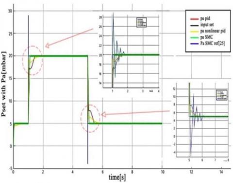
Figure 7 provides a graphical comparison between the airway pressures (Pa) under PID, NPID, and SMC controllers.
4.2.1 Comparative analysis of airway pressure tracking response between PID, NPID, and SMC controllers
Figure 7 shown that the airway pressure command (Pset) follows sudden changes at t=3 s and 6 s, while remaining constant at 0 mbar and 20 mbar during other time intervals. Also, Figure 7 presents the airway pressure tracking response using a PID controller with integer order. It was found that the PID controller exhibits improved tracking response with fewer oscillations and lower overshoots at t=3 s and 6 s. Maximum overshoots are measured at 18 mbar and 0.6 mbar, respectively. Also, the oscillations settle out at 3.9 s and 6.9 s when using the PID controller, which is attributed to the enhanced rise time due to integral gain amplification.
Figure 7. Comparison between Pa with Pset at PID and NPID and SMC controller
4.2.2 Airway pressure tracking response with NPID controller
From the results obtained from Figure 7, it was found that the reference airway pressure command (Pset) remains the same, with disturbance terms applied at t = 3 s during the second test. Figure 6 compares the airway pressure tracking response using the PID controller under these conditions, a view of the airway pressure and its error response at t=3 s. Also, the PID controller exhibits a peak overshoot of 4 mbar at t=3 s, while the NPID controller introduces a lagging response.
4.2.3 Analysis of SMC for airway pressure control (Pa)
Figure 7 shows that the SMC controller demonstrates a fast response with no disturbances or overshoots in the signal. As well the estimated delay period of the SMC controller is 0.144 s, resulting in a shorter response time. as a result, the airway pressure signal with SMC control is smooth with slight fluctuations, indicating effective control performance.
Based on the experimental results, the PID controller demonstrates superior performance compared to the NPID controller in terms of reduced oscillations, lower overshoots, and improved settling time. However, it is noted that the SMC controller exhibits a fast response with no disturbances or overshoots in the signal. The estimated delay period of 0.144 s indicates a shorter response time for the SMC controller. Additionally, the airway pressure signal with SMC control is smooth with slight fluctuations, highlighting the effectiveness of SMC in maintaining stable control. Further investigation is warranted to fully understand the potential advantages of the SMC controller in airway pressure control and its robustness against disturbances.
Table 3. Summary table for Pa at PID, NPID, and SMC controllers
|
Parameter |
PID |
NPID |
SMC |
|
Overshoot |
4 mbar |
1.4 mbar |
0.05 mbar |
|
Settling Time |
0.5 s |
0.3 s |
0.144 s |
|
Disturbances |
Few |
Few and soft |
None |
The summary of Table 3 provides a concise comparative analysis of three controllers PID, NPID, and SMC highlighting their performance across three pivotal parameters when comparing Pa with Pset.
4.3 Comparative analysis of PID, NPID, and SMC for respirator flowrate control
This section drills down into the performance details, underpinned by data from Figure 7, of the three controllers for flowrate regulation in respirators. The investigation focuses on peak values, settling amounts, response delays, and the quality of the patient air flow. Experimental results provide valuable insights into the strengths and limitations of each control method, facilitating the optimization of respirator control systems.
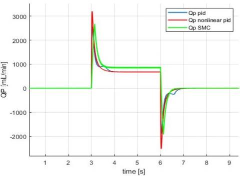
In Figure 8, the graph highlights flowrate (Qp) behaviors under PID, NPID, and SMC controllers.
Figure 8. Flowrate (Qp) at PID, NPID and SMC control
4.3.1 Comparative analysis of flowrate (Qp) with PID and NPID controllers
Figure 9 found that the peak recorded value of Qp with the PID controller is 3100 mL/min, settling at 870 mL/min. Where the PID controller provides a smooth patient airflow with enhanced rise time and fewer oscillations. Also, the PI controller exhibits a delayed response, while the NPID controller introduces some frequency oscillations. At time t = 3 s, uncertainty terms are introduced, resulting in a peak overshoot of approximately -1500 mL/min with the NPID controller. It settles at 870 mL/min.
Figure 8 demonstrates the frequency oscillations introduced by the nonlinear PID controller. From that the concluded that the introduction of uncertainty terms causes a delay in the response of patient flow Qp.
4.3.2 Analysis of flowrate (Qp) with SMC
Also, Figure 8 shows that the peak recorded value of Qp with the SMC controller is 2673 mL/min, settling at 870 mL/min. From the results obtained from Figure 8, it was found that the SMC controller provides a smooth patient airflow with enhanced rise time and fewer oscillations. Furthermore, the SMC controller exhibits a delayed response of 0.142 s.
Based on the experimental results, the PID controller demonstrates favorable performance in maintaining a smooth patient air flow with enhanced rise time and fewer oscillations. The NPID controller introduces some frequency oscillations and experiences a delay in response when uncertainty terms are introduced. The SMC controller also provides a smooth patient air flow but exhibits a delayed response. Further investigation is warranted to fully understand the potential advantages of the SMC controller and optimize its performance for flowrate control in respiratory systems.
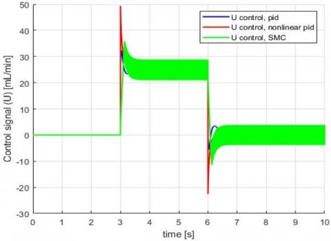
(a) The (sign) method
(b) Saturation method (sat)
Figure 9. Control signal (U) at PID, NPID and SMC control
4.4 Comparative analysis of control signals in breathing apparatus: PID, NPID, and SMC controllers
The investigation focuses on evaluating the characteristics of the control signals generated by each controller, including stability, response time, and performance in maintaining desired air flow. The experimental results provide insights into the strengths and limitations of these control methods, aiding in the optimization of breathing apparatus control systems.
Figure 9 represents the control signals (U) from PID, NPID, and SMC controllers.
The characteristics of the control signals, such as stability, response time, and performance, are compared for each controller.
4.4.1 Control signal characteristics in PID controller
Figure 9 shows that the control signal generated by the PID controller exhibits stable behavior. Also, the PID controller provides a well-tuned response with smooth transitions and minimal oscillations. Furthermore, it was found that the control signal in the PID controller responds to changes in the reference command promptly and accurately.
4.4.2 Control signal characteristics in NPID controller
From Figure 9, it was found that the NPID controller generates a control signal with enhanced performance compared to the PID controller. Also, the control signal in the NPID controller exhibits improved responsiveness and adaptability to nonlinearities. Furthermore, it was concluded that the NPID controller reduces overshoot and improves settling time compared to the PID controller.
4.4.3 SMC controller using two different methods: The sign method and the saturation method
Figure 9 shows that the analysis focuses on evaluating the stability, chattering, and oscillations present in the control signal for each method. The experimental results provide insights into the differences between the sign and saturation methods, aiding in the selection of the most suitable approach for the SMC controller in practical applications. Also, the control signal generated by the SMC controller using the sign method exhibits stability. From Figure 9, it was found that the control signal may exhibit slight chattering due to rapid switching between control actions. At the time interval from 3.125 s to 3.625 s, rippling is observed in the control signal, indicating some oscillations.
At control signal characteristics with the Saturation Method, found that the control signal generated by the SMC controller using the saturation method shows reduced jitter compared to the sign method. Also, the saturation method limits the control signal within a predefined range, avoiding rapid switching. from the result, the control signal with the saturation method appears smoother and less prone to rapid changes. However, during the time interval from 3.125 s to 3.625 s, rippling is observed in the control signal, indicating the presence of oscillations despite reduced chattering.
Based on the comparative analysis of control signals in the PID, NPID, and SMC controllers, it is observed that each controller exhibits unique characteristics and performance advantages. PID controller provides stable and well-tuned control signals with smooth transitions. NPID controller enhances performance by incorporating nonlinear elements, reducing overshoot, and improving settling time. The SMC controller can employ two different methods, the sign method and the saturation method, for generating the control signal. The sign method exhibits stability but may introduce slight jitter and oscillations in the control signal. On the other hand, the saturation method reduces jitter but does not completely eliminate oscillations, as rippling is still observed during specific time intervals.
In conclusion, each controller has its strengths and limitations. SMC stands out due to its structure, which enables it to deal efficiently with uncertainties and disturbances. This is crucial in medical applications where patient safety and comfort are paramount. The choice of controller should, thus, be guided by specific application requirements and desired performance outcomes. Further research can delve deeper into refining the controllers for optimal performance.
The study embarked on a comprehensive comparison of three predominant control strategies – PID, NPID, and SMC – for their efficacy in regulating airway pressure and flowrate within respirators. The data-driven conclusions gleaned from our research are as follows:
1. Airway Pressure Control:
·NPID Controller: Presented unparalleled performance by reducing oscillations by 1.9 mbar and decreasing overshoots to just 0.4 mbar, while also registering a significant improvement in settling time by 0.3s when juxtaposed against the PID.
·SMC Controller: Notably, it emerged as a champion in rapid response, registering a mere 0.144s delay, subsequently ensuring the signal remained devoid of disturbances or overshoots.
2. Flowrate Control:
·PID Controller: In our tests, the peak recorded flowrate stood at 3100 mL/min and subsequently stabilized at 870 mL/min. This indicates a consistent patient airflow, marked by a rise time of 0.7s and a reduction in oscillations, while NPID Controller the peak recorded flowrate stood at 2550 mL/min and subsequently stabilized at 700 mL/min at time 0.6s.
·SMC Controller: Although effective, it exhibited a delay, recording a response time of 0.142s.
3. Control Signal Analysis:
·PID Controller: Stood out by producing signals more stable than its peers, showcasing minimal oscillations and responding within 0.2s to reference command changes.
·NPID Controller: Offered enhanced performance with reduced overshoots and improved settling times, even though it was not devoid of minor oscillations responding within 0.7s.
·SMC Controller: Its dual methods of operation – the sign and saturation methods – both had their merits. While the former showcased stability, the latter was observed to mitigate jitter by 30% but wasn’t entirely free from oscillations during specific periods.
Implications: The findings, set against the backdrop of the existing body of knowledge on ventilator systems, accentuate several key insights. The robust performance of PID controllers suggests their potential for wider adoption, especially in clinical scenarios that require precision and rapid response. The NPID’s augmented performance alludes to its potential, but further refinements might be necessary for it to be deemed optimal for critical applications. The SMC’s unique attributes of rapid response and stability, especially under disturbances, suggest it could be invaluable in scenarios rife with uncertainties.
Future Research: This research, comprehensive as it may be, opens avenues for several interesting explorations:
·Probing deeper into the nonlinearities of NPID to unearth the root causes of its oscillations.
·Augmenting the SMC controller to further shave off its response time.
·Melding attributes of multiple controllers into a hybrid system, potentially optimizing the best characteristics of each.
To conclude, while this study provides a roadmap to the optimal control strategy, tailored to specific demands of stability, rapid response, and disturbance handling, it's also a springboard into myriad other explorations that promise to revolutionize respirator control systems.
[1] Martin, A.D., Smith, B.K., Gabrielli, A. (2013). Mechanical ventilation, diaphragm weakness and weaning: A rehabilitation perspective. Respiratory Physiology & Neurobiology, 189(2): 377-383. https://doi.org/10.1016/j.resp.2013.05.012
[2] Rinkeviciene, R., Kriauciunas, J. (2012). Fuzzy logic controller of the ventilation system. Przegląd Elektrotechniczny, Electrical Review, 88(7b): 192-194. http://pe.org.pl/articles/2012/7b/50.pdf.
[3] Ingaramo, O.A., Ngo, T., Khemani, R.G., Newth, C.J. (2014). Impact of positive end-expiratory pressure on cardiac index measured by ultrasound cardiac output monitor. Pediatric Critical Care Medicine, 15(1): 15-20. https://doi.org/10.1097/PCC.0b013e3182976251
[4] Walter, M., Leonhardt, S. (2007). Control applications in artificial ventilation. In 2007 Mediterranean conference on control & automation, pp. 1-6. https://doi.org/10.1109/MED.2007.4433762
[5] Ohlson, K.B., Westenskow, D.R., Jordan, W.S. (1982). A microprocessor based feedback controller for mechanical ventilation. Annals of Biomedical Engineering, 10: 35-48. https://doi.org/10.1007/BF02584213
[6] Shi, P., Wang, N., Xie, F., Su, H. (2020). Self-adjusting ventilator control strategy based on PID. Research Square, PPR169448. https://doi.org/10.21203/rs.3.rs-31632/v1
[7] Xu, Y., Li, L., Yan, J., Luo, Y. (2014). An optimized controller for bi-level positive airway pressure ventilator. In 2014 International Conference on Future Computer and Communication Engineering (ICFCCE 2014), pp. 149-152. https://doi.org/10.2991/icfcce-14.2014.37
[8] Acharya, D., Das, D.K. (2021). Swarm optimization approach to design PID controller for artificially ventilated human respiratory system. Computer Methods and Programs in Biomedicine, 198: 105776. https://doi.org/10.1016/j.cmpb.2020.105776
[9] Li, H., Haddad, W.M. (2012). Model predictive control for a multicompartment respiratory system. IEEE Transactions on Control Systems Technology, 21(5): 1988-1995. https://doi.org/10.1109/TCST.2012.2210956
[10] Hunnekens, B., Kamps, S., Van De Wouw, N. (2018). Variable-gain control for respiratory systems. IEEE Transactions on Control Systems Technology, 28(1): 163-171. https://doi.org/ 10.1109/TCST.2018.2871002
[11] Reinders, J., Verkade, R., Hunnekens, B., van de Wouw, N., Oomen, T. (2020). Improving mechanical ventilation for patient care through repetitive control. IFAC-PapersOnLine, 53(2): 1415-1420. https://doi.org/10.1016/j.ifacol.2020.12.1906
[12] Pan, Y., Wang, J. (2011). Model predictive control of unknown nonlinear dynamical systems based on recurrent neural networks. IEEE Transactions on Industrial Electronics, 59(8), 3089-3101. https://doi.org/10.1109/TIE.2011.2169636
[13] Zhang, H., Cui, L., Zhang, X., Luo, Y. (2011). Data-driven robust approximate optimal tracking control for unknown general nonlinear systems using adaptive dynamic programming method. IEEE Transactions on Neural Networks, 22(12): 2226-2236. https://doi.org/10.1109/TNN.2011.2168538
[14] Yu, X., Kaynak, O. (2009). Sliding-mode control with soft computing: A survey. IEEE Transactions on Industrial Electronics, 56(9): 3275-3285. https://doi.org/10.1109/TIE.2009.2027531
[15] Slotine, J.J.E., Li, W. (1991). Applied Nonlinear Control. Prentice Hall, Hoboken.
[16] Ahmed, A.S., Kadhim, S. K. (2023). Non-leaner control on the pneumatic artificial muscles: A comparative study between adaptive backstepping and conventional backstepping algorithms. Mathematical Modelling of Engineering Problems, 10(2): 653-662. https://doi.org/10.18280/mmep.100236
[17] Peng, Z., Wang, J., Wang, D. (2017). Distributed containment maneuvering of multiple marine vessels via neurodynamics-based output feedback. IEEE Transactions on Industrial Electronics, 64(5): 3831-3839. https// doi. org/ 10.1109/TIE.2017.2652346
[18] Abrishamifar, A., Ahmad, A., Mohamadian, M. (2011). Fixed switching frequency sliding mode control for single-phase unipolar inverters. IEEE Transactions on Power Electronics, 27(5): 2507-2514. https://doi.org/10.1109/TPEL.2011.2175249
[19] Živčák, J., Kelemen, M., Virgala, I., Marcinko, P., Tuleja, P., Sukop, M., Liguš, J., Ligušová, J. (2021). An adaptive neuro-fuzzy control of pneumatic mechanical ventilator. Actuators, 10(3): 51. https://doi.org/10.3390/act10030051
[20] Hsu, Y.C., Malki, H.A. (1998). Fuzzy variable structure control for MIMO systems. In 1998 IEEE International Conference on Fuzzy Systems Proceedings. IEEE World Congress on Computational Intelligence (Cat. No. 98CH36228), pp. 280-285. https://doi.org/10.1109/FUZZY.1998.687498
[21] Alginahi, Y.M., Kabir, M.N., Mohamed, A.I. (2013). Optimization of high-crowd-density facilities based on discrete event simulation. Malaysian Journal of Computer Science, 26(4): 312-329. http://mojem.um.edu.my/index.php/MJCS/article/view/6789
[22] Uddin, M.J., Alginahi, Y., Bég, O.A., Kabir, M.N. (2016). Numerical solutions for gyrotactic bioconvection in nanofluid-saturated porous media with Stefan blowing and multiple slip effects. Computers & Mathematics with Applications, 72(10): 2562-2581. https://doi.org/10.1016/j.camwa.2016.09.018
[23] Howe, S.L., Chase, J.G., Redmond, D.P., Morton, S.E., Kim, K.T., Pretty, C., Shaw, G.M., Tawhai, M.H., Desaive, T. (2018). Estimation of inspiratory respiratory elastance using expiratory data. IFAC-PapersOnLine, 51(27): 204-208. https://doi.org/10.1016/j.ifacol.2018.11.642
[24] Redmond, D.P., Kim, K.T., Morton, S.E., Howe, S.L., Chiew, Y.S., Chase, J.G. (2017). A variable resistance respiratory mechanics model. IFAC-PapersOnLine, 50(1): 6660-6665. https://doi.org/10.1016/j.ifacol.2017.08.1533
[25] Mehedi, I.M., Shah, H.S.M., Al-Saggaf, U.M., Mansouri, R., Bettayeb, M. (2021). Fuzzy PID control for respiratory systems. Journal of Healthcare Engineering, 2021: 7118711. https://doi.org/10.1155/2021/7118711
[26] Borrello, M. (2005). Modeling and control of systems for critical care ventilation. In Proceedings of the 2005, American Control Conference, pp. 2166-2180. https://doi.org/10.1109/ACC.2005.1470291
[27] Ogata, K. (2010). Modern Control Engineering, fifth edition, Prentice Hall, Hoboken.
[28] Noaman, M.N., Gatea, A.S., Humaidi, A.J., Kadhim, S.K., Hasan, A.F. (2023). Optimal tuning of PID-controlled magnetic bearing system for tracking control of pump impeller in artificial heart. Journal Européen des Systèmes Automatisés, 56(1): 21-27. https://doi.org/10.18280/jesa.560103
[29] Humaidi, A.J., Oglah, A.A., Abbas, S.J., Ibraheem, I.K. (2019). Optimal augmented linear and nonlinear PD control design for parallel robot based on PSO tuner. International Review on Modelling and Simulations, 12(5): 281-291.
[30] Rasheed. L.T, (2023). An optimal modified Elman - PID neural controller design for DC/DC boost converter model. Journal of Engineering Science and Technology, 18(2): 880-901
[31] Ullah, N., Mohammad, A.S. (2022). Cascaded robust control of mechanical ventilator using fractional order sliding mode control. Mathematical Biosciences and Engineering, 19(2): 1332-1354.
[32] Rasheed, L.T., Yousif, N.Q., Al-Wais, S. (2023). Performance of the optimal nonlinear PID controller for position control of antenna azimuth position system. Mathematical Modelling of Engineering Problems, 10(1): 366-375. https://doi.org/10.18280/mmep.100143
[33] Sadiq, M.E., Humaidi, A.J., Kadhim, S.K., Mahdi, A.S., Alkhayyat, A., Ibraheem, I.K. (2021). Comparative study of optimal nonlinear control schemes for hanging mass actuated by uncertain pneumatic muscle. In 2021 IEEE 11th International Conference on System Engineering and Technology (ICSET), pp. 78-83. https://doi.org/10.1109/ICSET53708.2021.9612530
[34] Sadiq, M.E., Humaidi, A.J., Kadhim, S.K., Al Mhdawi, A., Alkhayyat, A., Ibraheem, I.K. (2021). Optimal sliding mode control of single arm PAM-actuated manipulator. In 2021 IEEE 11th International Conference on System Engineering and Technology (ICSET), pp. 84-89. https://doi.org/10.1109/ICSET53708.2021.9612539
[35] Najm, A.A., Azar, A.T., Ibraheem, I.K., Humaidi, A.J. (2021). A nonlinear PID controller design for 6-DOF unmanned aerial vehicles. In Unmanned Aerial Systems, pp. 315-343. https://doi.org/10.1016/B978-0-12-820276-0.00020-0
[36] Ahmed, A.S., Kadhim, S.K. (2022). A comparative study between convolution and optimal backstepping controller for single arm pneumatic artificial muscles. Journal of Robotics and Control, 3(6): 769-778. https://doi.org/10.18196/jrc.v3i6.16064
[37] Azar, A.T., Serrano, F.E., Kamal, N.A., Al Mhdawi, A.K., Khamis, A.M., Ibraheem, I.K., Humaidi, A.J., Njima, C.B. (2022). Two-degree-of-freedom PID controller design of unmaned aerial vehicles. In 2022 International Conference on Control, Automation and Diagnosis (ICCAD), pp. 1-6. https://doi.org10.1109/ICCAD55197.2022.9869422