Sutrisno Sutrisno*![]() | Widowati Widowati
| Widowati Widowati![]() | Sunarsih Sunarsih
| Sunarsih Sunarsih![]() | Kartono Kartono
| Kartono Kartono![]() | Purnawan Adi Wicaksono
| Purnawan Adi Wicaksono![]() | Tosporn Arreeras
| Tosporn Arreeras![]() | Muhammad Syukur
| Muhammad Syukur![]()
© 2023 IIETA. This article is published by IIETA and is licensed under the CC BY 4.0 license (http://creativecommons.org/licenses/by/4.0/).
OPEN ACCESS
This study addresses the integration of supplier selection and inventory management issues that involve discounts, with a unified decision-making support formulated through a mathematical programming approach. The challenges addressed encompass uncertain parameters such as defective goods rates, late delivery rates, and demand, some of which are treated as probabilistic/random variables under data availability assumptions, while others are managed as fuzzy variables where data is not explicitly required. The joint problems were synthesized into a piecewise fuzzy-probabilistic optimization model with the aim of minimizing total operational costs, and the optimal decision was deduced by solving this model. Further, the model was constructed incorporating multi-period observations, indicating its ability to generate optimal solutions for multiple procurement activity periods. Computational simulations were executed to demonstrate the calculation of the optimal decision and to appraise the proposed model. All calculations were performed in LINGO 19.0 optimization software, leveraging its uncertain programming package. The computational process employed the generalized reduced gradient - a popular method for solving optimization problems due to its requirement of only a differentiable objective function - in conjunction with the branch and bound algorithm - recognized for its simplicity in branching and bounding feasible solutions. The results affirmed that the proposed model successfully delivered the optimal solution for the problem at hand. Therefore, the proposed model is deemed appropriate for implementation by practitioners in manufacturing/retail industries as a decision-making tool to curtail operational costs associated with their procurement and warehousing operations.
discounts, fuzzy-probabilistic programming, inventory management, piecewise optimization, supplier selection, supply chain
Decision-makers in manufacturing and retail industries have been continuously attempting to optimize all supply-chain activities in order to generate larger profit. Optimizing the whole supply-chain problems simultaneously from the upstream parties such as raw material suppliers up to the downstream parties such as buyers is impossible due to the extensive size of the problems. In many cases, decision-makers divide supply-chain problems into supply-chain activities and optimize them independently or in an integrated manner for some inter-connected activities.
Numerous approaches, mostly in mathematical model forms, have been proposed to optimize certain problems in supply chain independently. For supplier selection problems, some pioneering models can be found in the study [1]. Monteiro et al. [2] dealt with simpler problem specifications, e.g., there are no discounts, and all parameters are certain. Generally, more complex specifications lead to more complex models. For instance, more complex models have been proposed in Wicaksono [3] and Widowati [4] to address supplier selection problems under full truckload transportation schemes. Models with price discounts are built in the studies [5, 6], however, all involved parameters are certain. Cases with uncertain parameters in the form of probabilistic and fuzzy were constructed in this study to fill the prevalent research gap. Numerous studies have been carried out in dealing with supplier selection problems, indicating the need of decision-making support for such problems in many fields such as power management [7-9], healthcare [10, 11], automotive [12, 13], electrical equipment manufacturing [14, 15], garment industries [16], mega-construction [17], and others.
Several mathematical models have also been proposed to solve inventory management problems independently. For example, in the studies [18-20], three models have been proposed to solve inventory under sales dependent stochastic return flows, carbon emissions policies, and with varying perishability rate product, respectively. Another approach has been proposed using deep reinforcement learning in the study [21]. However, there were no integrations with other parties such as suppliers. Various studies that had been conducted emphasize the need of inventory models in real world problems such as pharmaceutical inventory [22], textile industries [23], grocery retail [24], and many more. In particular, case studies that contain uncertain parameters can be found in numerous reports from various fields such as supply chain management [25], mechanical devices [26, 27], and transportation [28], further demonstrating that uncertain parameters naturally occur in real world problems.
To address the aforementioned supplier selection and inventory management problems in an integrated manner, some models have been proposed in previous studies such as two models in the studies [5, 6]. However, all parameters were fully certain, and no model has been constructed under uncertainty, especially with both probabilistic and fuzzy variables; this is the main weakness of the existing studies and will be resolved in this paper. Furthermore, uncertain parameters naturally occur in real-world problems. Probabilistic parameters can be used to treat parameters with historical data. Nevertheless, the trend of the data may change, and when data do not represent the reality anymore, fuzzy parameters can be used to treat the corresponding parameters. This leads to the need of having both probabilistic and fuzzy parameters in the decision-making processes. Therefore, this study aimed to propose a joint decision-making support for integrated supplier selection and inventory management involving discounts, probabilistic parameters, and fuzzy parameters. The proposed model is in the form of fuzzy-probabilistic programming and is demonstrated via computational simulations. The discounts are in piecewise constant forms whereas the probabilistic parameters have normal probability distribution functions, and the fuzzy parameters have discrete membership functions; those approaches are commonly used in practice due to their simplicity in formulating the corresponding price or probability or membership functions.
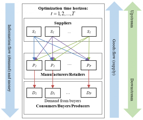
Figure 1. The supply chain flow
2.1 Problem setting
Consider the supply chain illustrated by Figure 1. When a manufacturer or retail company needs to purchase goods from several suppliers, not all suppliers might need to be selected; only some would be eventually selected. Furthermore, the scenario also involves several types of goods which will be handled simultaneously. A particular supplier might only supply certain types of goods. Therefore, the problem is to determine an optimal decision in determining the quantities of goods that should be purchased to each supplier such that the procurement cost is minimal and the demand is satisfactorily fulfilled. Moreover, when multi-period optimizations are considered, decision-makers wish to find optimal decisions from multiple observations.
The problem becomes more complicated as some goods could be stored in the inventory between two consecutive observation periods, which can be used to fulfill the demand in the future time periods. In addition, decision-makers should determine the quantity of goods that should be stored in the inventory for each type of goods, and the optimal decision should also minimize the total holding cost along the observation time horizon.
The particular specification considered in this problem is that suppliers provide price discounts for their goods. Transportation costs and holding costs also involve discounts. Meanwhile, some parameters are uncertain, hence creating more complicated problems.
To be precise, the problem specifications as well as the assumptions adopted in the problem-solving process are as follows:
2.2 Problem solving procedure
The methodology implemented in this study is summarized in Figure 2 with explanation as follows. In step 1, the problem was identified as described in the problem setting. The functions of prices/costs with discounts were in piecewise constant functions (see mathematical model for further details). In step 2, the uncertain parameters could be either probabilistic or fuzzy. For probabilistic parameters, the probability distribution function was formulated from the (historical or trial) data. Otherwise, decision-makers formulated its membership function based on intuition and observation/experience. The discrete membership function was adopted in this study (see mathematical model for further explanation).
Figure 2. The supply problem solving procedure
Step 3 included mathematical symbol declaration, cost component formulation, and each constraint function based on assumptions and conditions from the problem. In step 4, all computations were carried out in LINGO 19.0 optimization software. The uncertain programming package was utilized, and the generalized reduced gradient algorithm was used in running the computations. To obtain integer solutions, the branch-and-bound method was employed. LINGO was chosen due to its flexibility on solving optimization problems. Any kind of objective functions and constraint functions can be added to the problem, and it can detect the type of the optimization problem. Furthermore, it can also handle many kinds of optimization problems including uncertain programming, for further technical details, one may refer [29]. Meanwhile, the generalized reduced gradient combined with branch and bound was chosen since it has been reported as one of the most popular methods to solve optimization problems, see, e.g., the study [30]. One of the main advantages of it is that it only requires the objective function to be differentiable. In particular, branch-and-bound scheme is a well-known method for finding integer solutions by simply branching and bounding the feasible solutions [31].
In solving uncertain programming, the model was first converted into its deterministic equivalent programming by considering the expectation values for the objective and constraint functions. Subsequently, it was solved using algorithms for certain programming. The theoretical studies regarding uncertain programming are highlighted in the study [32]. In step 5, the optimal decision generated by the proposed decision-making support was eventually implemented. It should be noted that multiple computations could be run in the event that the generated decisions are unsatisfactory since the calculations are carried out under uncertainty. Therefore, computations can be re-run with different values such as different membership functions for the fuzzy parameters.
The notations used in the mathematical modeling process of the decision-making support are available in the Nomenclature section at the end of the paper. The decision variables, semi-decision variables (values that follow the decision variables), uncertain parameters, and the certain parameters are also listed in the Nomenclature section. First, we introduce in the following the discounted prices/costs functions, which are in piecewise constant functions:
$U P_{t s p}= \begin{cases}U P_{t s p}^{(1)} & \text { if } \mathcal{X}_{t s p} \leq \mathcal{X}_{t s p}^{(1)}, \\ U P_{t s p}^{(2)} & \text { if } \mathcal{X}_{t s p}^{(1)}<\mathcal{X}_{t s p} \leq \mathcal{X}_{t s p}^{(2)}, \\ \vdots & \\ U P_{t s p}^{(\hat{i})} & \text { if } \quad \mathcal{X}_{t s p}>\mathcal{X}_{t s p}^{(\hat{i}-1)} ;\end{cases}$ (1)
$T C_{t s}=\left\{\begin{array}{lll}T C_{t s}^{(1)} & \text { if } & \mathcal{T}_{t s} \leq \mathcal{T}_{t s}^{(1)}, \\ T C_{t s}^{(2)} & \text { if } & \mathcal{T}_{t s}^{(1)}<\mathcal{T}_{t s} \leq \mathcal{T}_{t s}^{(2)}, \\ \vdots & & \\ T C_{t s}^{(\hat{j})} & \text { if } & \mathcal{T}_{t s}>\mathcal{T}_{t s}^{(\hat{j}-1)}.\end{array}\right.$ (2)
$I C_{t p}= \begin{cases}I C_{t p}^{(1)} & \text { if } \mathcal{I}_{t p} \leq \mathcal{I}_{t p}^{(1)}, \\ I C_{t p}^{(2)} & \text { if } \mathcal{I}_{t p}^{(1)}<\mathcal{I}_{t p} \leq \mathcal{I}_{t p}^{(2)}, \\ \vdots & \\ I C_{t p}^{(\hat{k})} & \text { if } \mathcal{I}_{t p}>\mathcal{I}_{t p}^{(\hat{k}-1)}.\end{cases}$ (3)
The above piecewise constant functions of prices/costs represent the discount schemes in which more goods/services provide cheaper prices/costs, which are common in industries. Each price level is separated by breakpoints, which are determined by the goods/services provider.
The target of the optimization is the total operational cost, which includes the following cost components:
$Z_1=\sum_{t=1}^T \sum_{s=1}^S\left[O C_{t s} \times \mathcal{Y}_{t s}\right].$ (4)
$Z_2=\left\{\begin{array}{l}\sum_{t=1}^T \sum_{s=1}^S \sum_{p=1}^P\left[U P_{t s p}^{(1)} \times \mathcal{X}_{t s p}\right] \\ \text { if } \mathcal{X}_{t s p} \leq \mathcal{X}_{t s p}^{(1)}, \\ \sum_{t=1}^T \sum_{s=1}^S \sum_{p=1}^P\left[U P_{t s p}^{(2)} \times \mathcal{X}_{t s p}\right] \\ \text { if } \mathcal{X}_{t s p}^{(1)}<\mathcal{X}_{t s p} \leq \mathcal{X}_{t s p}^{(2)}, \\ \vdots \\ \sum_{t=1}^T \sum_{s=1}^S \sum_{p=1}^P\left[U P_{t s p}^{(\hat{i})} \times \mathcal{X}_{t s p}\right] \\ \text { if } \mathcal{X}_{t s p}>\mathcal{X}_{t s p}^{(\hat{i}-1)} .\end{array}\right.$ (5)
$Z_3=\left\{\begin{array}{l}\sum_{t=1}^T \sum_{s=1}^S\left[T C_{t s}^{(1)} \times \mathcal{T}_{t s}\right] \text { if } \mathcal{T}_{t s}^{(0)} \leq \mathcal{T}_{t s} \leq \mathcal{T}_{t s}^{(1)}, \\ \sum_{t=1}^T \sum_{s=1}^S\left[T C_{t s}^{(2)} \times \mathcal{T}_{t s}\right] \text { if } \mathcal{T}_{t s}^{(1)} \leq \mathcal{T}_{t s} \leq \mathcal{T}_{t s}^{(2)}, \\ \vdots \\ \sum_{t=1}^T \sum_{s=1}^S\left[T C_{t s}^{(\hat{j})} \times \mathcal{T}_{t s}\right] \text { if } \mathcal{T}_{t s}^{(\hat{j}-1)} \leq \mathcal{T}_{t s} \leq \mathcal{T}_{t s}^{(\hat{j})}.\end{array}\right.$ (6)
$Z_4=\sum_{t=1}^T \sum_{s=1}^S \sum_{p=1}^P\left[\mathcal{P}_{t s p}^{\mathcal{L}} \times \overline{\overline{\mathcal{L}}}_{t s p} \times \mathcal{X}_{t s p}\right].$ (7)
$Z_5=\sum_{t=1}^T \sum_{s=1}^S \sum_{p=1}^P\left[\mathcal{P}_{t s p}^{\mathcal{D}} \times \overline{\overline{\mathcal{D}}}_{t s p} \times \mathcal{X}_{t s p}\right].$ (8)
$Z_6=\sum_{t=1}^T \sum_{p=1}^P\left[R C_{t p} \times \mathcal{R}_{t p}\right].$ (9)
$Z_7= \begin{cases}\sum_{t=1}^T \sum_{p=1}^P\left[I C_{t p}^{(1)} \times \mathcal{I}_{t p}\right] & \text { if } \mathcal{I}_{t p} \leq \mathcal{I}_{t p}^{(1)}, \\ \sum_{t=1}^T \sum_{p=1}^P\left[I C_{t p}^{(2)} \times \mathcal{I}_{t p}\right] & \text { if } \mathcal{I}_{t p}^{(1)}<\mathcal{I}_{t p} \leq \mathcal{I}_{t p}^{(2)}, \\ \vdots & \\ \sum_{t=1}^T \sum_{p=1}^P\left[I C_{t p}^{(\hat{k})} \times \mathcal{I}_{t s p}\right] & \text { if } \mathcal{I}_{t p}>\mathcal{I}_{t p}^{(\hat{k}-1)} .\end{cases}$ (10)
$Z_8=\sum_{s=1}^S\left[C C_s \times \mathcal{Z}_s\right].$ (11)
The constraint functions that need to be satisfied were subsequently formulated based on the assumptions and conditions described in the problem statement. The constraint functions are formulated as follows:
$\begin{gathered}\mathcal{I}_{(t-1) p}+\sum_{s=1}^S \mathcal{X}_{t s p}+\sum_{s=1}^S\left[\overline{\overline{\mathcal{L}}}_{(t-1) s p} \times \mathcal{X}_{(t-1) s p}\right] -\sum_{s=1}^S\left[\overline{\overline{\mathcal{L}}}_{t s p} \times \mathcal{X}_{t s p}\right]-\sum_{s=1}^S\left[\overline{\overline{\mathcal{D}}}_{t s p} \times \mathcal{X}_{t s p}\right]+\mathcal{R}_{t p} \geq \mathbb{D}_{t p}, \\ \forall t=1,2, \ldots, T, \forall p=1,2, \ldots, P;\end{gathered}$ (12)
where, $\mathcal{I}_{(0) p}$ is the initial inventory level for goods p; commonly, it is zero if no goods are available in the warehouse at the initial time, and $\overline{\overline{\mathcal{L}}}_{(0) s p}$ is zero as no goods was purchased before the initial time. If the inventory is initially not empty, then $\mathcal{I}_{(0) p}$ can be set to be nonzero. This inequality is used to ensure that the demand is expected to be always satisfied.
$\sum_{p=1}^P \mathcal{X}_{t s p} \leq T R C \times \mathcal{T}_{t s}, \quad \forall t=1,2, \ldots, T, \forall s=1,2, \ldots, S.$ (13)
This is needed to calculate the number of deliveries which is used to calculate the transportation cost.
$\mathcal{Y}_{t s}=\left\{\begin{array}{ll}1 & \text { if } \sum_{p=1}^P \mathcal{X}_{t s p}>0, \\ 0 & \text { otherwise; }\end{array} \quad \forall t=1,2, \ldots, T, \forall s=1,2, \ldots, S.\right.$ (14)
This constraint function is used to determine whether a supplier is selected or not at a particular time observation period and is used to calculate the order cost at every time observation period in the objective function.
$\mathcal{Z}_s=\left\{\begin{array}{ll}1 & \text { if } \sum_{t=1}^T \sum_{p=1}^P \mathcal{X}_{t s p}>0, \\ 0 & \text { otherwise; }\end{array} \quad \forall s=1,2, \ldots, S ;\right.$ (15)
or, alternatively,
$\mathcal{Z}_s=\left\{\begin{array}{ll}1 & \text { if } \sum_{t=1}^T \mathcal{Y}_{t s}>0, \\ 0 & \text { otherwise; }\end{array} \quad \forall s=1,2, \ldots, S.\right.$ (16)
This binary variable is utilized to determine whether a supplier is selected or not for the whole planning time horizon and is used to calculate the contract cost in the objective function.
$\begin{gathered}\mathcal{X}_{t s p} \leq S C_{t s p}, \quad \forall t=1,2, \ldots, T, \forall s=1,2, \ldots, S, \\ \forall p=1,2, \ldots, P .\end{gathered}$ (17)
This bound is rather obvious as suppliers have maximum capacity limits in supplying goods, and this constraint is used to ensure that the decision in ordering goods does not excess the maximum number of goods can be provided by suppliers. If a supplier does not have a capacity limit, the upper bound can be simply set as a sufficiently big number; this will imply that the feasible region of the optimization problem is bounded.
$\mathcal{I}_{t p} \leq M I_{t p}, \quad \forall t=1,2, \ldots, T, \forall p=1,2, \ldots, P;$ (18)
Similar to upper bounds for suppliers, this is used to make sure that the number of goods stored in the warehouses does not excess its maximum capacity limits.
$\mathcal{X}_{t s p}, \mathcal{T}_{t s}, \mathcal{I}_{t p} \geq 0$ and integer, $\forall t=1,2, \ldots, T, \forall s=1,2, \ldots, S, \forall p=1,2, \ldots, P.$ (19)
The nonnegativity constraints are obvious since all decision variables have to be nonnegative. The integer constraints are optional; some variables related to particular goods may be non-integer if their measurements follow real numbers.
Since the problem contains uncertain parameters, the expectation value of the total operational cost was minimized instead of its actual value. This is due to the presence of probabilistic and fuzzy parameters, and thus the actual value cannot be known before those uncertain parameters are revealed; and the decision-maker can only expect the operational cost. Subsequently, as a complete mathematical optimization problem, the proposed model was rewritten a`s follows:
$\min _{\mathcal{X}_{t s p}, \,\mathcal{I}_{t p}, \mathcal{R}_{t p}} Z=\mathcal{E}\left[\sum_{l=1}^8 Z_l\right]$ (20)
subject to:
$\begin{gathered}\mathcal{E}\left[\mathcal{I}_{(t-1) p}+\sum_{s=1}^S \mathcal{X}_{t s p}+\sum_{s=1}^S\left[\overline{\overline{\mathcal{L}}}_{(t-1) s p} \times \mathcal{X}_{(t-1) s p}\right]\right. \left.-\sum_{s=1}^S\left[\overline{\overline{\mathcal{L}}}_{t s p} \times \mathcal{X}_{t s p}\right]-\sum_{s=1}^S\left[\overline{\overline{\mathcal{D}}}_{t s p} \times \mathcal{X}_{s p}\right]+\mathcal{R}_{t p}-\mathbb{D}_{t p}\right] \geq 0 \\ \forall t=1,2, \ldots, T, \forall p=1,2, \ldots, P;\end{gathered}$ (21)
$\sum_{p=1}^P \mathcal{X}_{t s p}-T R C \times \mathcal{T}_{t s} \leq 0, \quad \forall t=1,2, \ldots, T, \forall s=1,2, \ldots, S;$ (22)
$\mathcal{Y}_{t s}=\left\{\begin{array}{ll}1 & \text { if } \sum_{p=1}^P \mathcal{X}_{t s p}>0, \\ 0 & \text { otherwise; }\end{array} \forall t=1,2, \ldots, T, \forall s=1,2, \ldots, S;\right.$ (23)
$\mathcal{Z}_s=\left\{\begin{array}{ll}1 & \text { if } \sum_{t=1}^T \mathcal{Y}_{t s}>0, \\ 0 & \text { otherwise; }\end{array} \quad \forall s=1,2, \ldots, S;\right.$ (24)
$\begin{gathered}\mathcal{X}_{t s p} \leq S C_{t s p}, \quad \forall t=1,2, \ldots, T, \forall s=1,2, \ldots, S, \forall p=1,2, \ldots, P;\end{gathered}$ (25)
$\mathcal{I}_{t p} \leq M I_{t p}, \quad \forall t=1,2, \ldots, T, \forall p=1,2, \ldots, P;$ (26)
$\mathcal{X}_{t s p}, \mathcal{T}_{t s}, \mathcal{I}_{t p} \geq 0$ and integer, $\forall t=1,2, \ldots, T, \forall s=1,2, \ldots, S, \forall p=1,2, \ldots, P.$ (27)
Note that this optimization problem involves uncertain parameters, some of them are probabilistic with some known probability distribution functions such as normal distribution and some others are fuzzy with some known membership functions such as discrete membership function. This optimization problem belongs to uncertain programming, and the technique used to solve it in this paper is based on the uncertain programming method provided in the study [33]. The general steps to solve are is first, the uncertain optimization problem is converted as a deterministic-equivalent optimization model by utilizing the probability distribution functions of the probabilistic parameters and the membership functions of the fuzzy parameters. Then, the optimization algorithms are employed to calculate the optimal decision from the deterministic equivalent model. For technical details, one may refer to [29, 33]. Furthermore, it should be also noted that the objective function is in a piecewise function since it is a piecewise function of discounted prices/costs. Therefore, the above optimization problem is in a piecewise programming class. From all constraint functions, the decision variables’ feasible region is closed as bounded. Provided that it is not empty, then an optimal decision is guaranteed to exist. Hence, the mathematical optimization in Eq. (20) is well defined.
To illustrate how the proposed model works, and to evaluate the mathematical model, computational simulations were performed. All tests were carried out in a personal computer with common specifications (3.0 GHz of processor and 8 GB of RAM) and all data were randomly generated using the function “@SPDISTNORM” in LINGO 19.0 for probabilistic parameters, and the function “RANDBETWEEN” in Ms Excel Software for realization values of fuzzy parameters.
4.1 Computational experiments setup
The optimization model in Eq. (20) was solved with five suppliers S1, S2, S3, S4, and S5, three types of goods P1, P2, and P3, three discount levels/price break points DL1, DL2, and DL3, and six observation time periods. There were three discounted prices/costs, namely unit prices of goods, delivery costs, and holding/inventory costs given by the following price functions:
$U P_{t s p}= \begin{cases}U P_{t p}^{(1)} \text { if } \mathcal{X}_{s p} \leq 5, \\ U P_{t p}^{(2)} \text { if } 5<\mathcal{X}_{p p} \leq 15, \\ U P_{t p}^{(3)} \text { if } \mathcal{X}_{s p}>15;\end{cases}$
$T C_{t s}=\left\{\begin{array}{l}T C_{t s}^{(1)} \text { if } \mathcal{T}_{t s} \leq 2, \\ T C_{t s}^{(2)} \text { if } 2<\mathcal{T}_{t s} \leq 5, \\ T C_{t s}^{(3)} \text { if } \mathcal{T}_{t s}>5;\end{array}\right.$
$I C_{t p}=\left\{\begin{array}{l}I C_{t p}^{(1)} \text { if } \mathcal{I}_{t p} \leq 10, \\ I C_{t p}^{(2)} \text { if } 10<\mathcal{I}_{t p} \leq 15, \\ I C_{t p}^{(3)} \text { if } \mathcal{I}_{t p} 15;\end{array}\right.$
where the values for $U P_{t s p}^{(i)}$, $T C_{t s}^{(j)}$, and $I C_{t p}^{(k)}$ are listed in the appendix. For uncertain parameters, the demand was fuzzy with the following discrete membership functions:
$F_{\overline{\bar{D}}_p}= \begin{cases}0.10 \text { if } \overline{\overline{\mathbb{D}}}_{t p}=30, & 0.85 \text { if } \overline{\overline{\mathbb{D}}}_{t p}=55, \\ 0.20 \text { if } \overline{\overline{\mathbb{D}}}_{t p}=35, & 1.00 \text { if } \overline{\overline{\mathbb{D}}}_{t p}=60, \\ 0.40 \text { if } \overline{\overline{\mathbb{D}}}_{t p}=40, & 0.75 \text { if } \overline{\overline{\mathbb{B}}}_{t p}=65, \\ 0.55 \text { if } \overline{\overline{\mathbb{D}}}_{t p}=45, & 0.50 \text { if } \overline{\overline{\mathbb{D}}}_{t p}=70, \\ 0.75 \text { if } \overline{\overline{\mathbb{D}}}_{t p}=50, & 0.25 \text { if } \overline{\overline{\mathbb{D}}}_{t p}=75 ;\end{cases}$
whereas the rejection and late delivery rates had normal/Gaussian distributions with 7.5% and 5% of mean, respectively, and 1% of standard deviation for both parameters. The distributions were applied for all observation time periods, all suppliers, and all goods. At the initial time, the initial inventory level was assumed to be zero, i.e., no goods were stored in the warehouse. The values of remaining parameters are listed in the appendix.
4.2 Results
The optimal decisions regarding procurement and inventory are shown in Figures 3 and 4. The proposed model generated this solution to achieve the smallest expectation value of the total operational cost, including the total holding cost for all goods for all time periods. The expected total operational cost was 33,582.903.
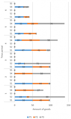
Figure 3. Optimal decisions for the product volume to be ordered
Only three out of five suppliers were selected along the optimization time horizon 1 to 6 (suppliers S1, S2 and S4), therefore the contract costs only applied to those suppliers. However, not all those selected suppliers were selected at each time period. For example, at time period 2, only S1 and S4 were selected since purchasing goods from those two suppliers was expected to be sufficient in satisfying the demand. In particular, selecting suppliers S1 and S4 provides the minimal procurement cost and buying goods from other suppliers may increase the procurement cost. Furthermore, not all goods types were purchased from each selected supplier. For instance, only goods P1 and P3 were purchased from supplier S1 at time period 6. This decision provides the minimal procurement cost since, mathematically, the procurement cost may be bigger if those goods are bought from other supplier. It shows that the optimal decision is indeed not obvious, and a decision-making support is needed. Furthermore, the proposed model successfully solved the given supply chain problem and provided the optimal solution.
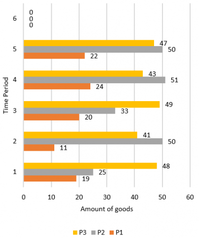
Figure 4. Optimal decisions regarding the inventory management
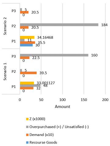
Figure 5. Demand values and their corresponding recourse product volume for multiple scenarios
The optimal decision related to the inventory management is shown in Figure 4. It should be noted that at time period 1, the initial inventory was zero, meaning that the demand was fully satisfied by the purchased goods at that time period. From Figure 4, it can be seen that certain quantities for each goods type were decided to be stored in the inventory. However, at time period 6, it was decided to not store goods in the warehouse since this was the last time period of the optimization, and thus storing goods was not necessary.
It was observed that the decisions were calculated under uncertainty of several parameters and were executed before decision-makers were aware of the actual values of those uncertain parameters. This means that after all values of uncertain parameters at past time periods are revealed, the actual operational cost may differ from the one generated by the decision-making support. It also means that the demand at the current time period could be not fully satisfied. Figure 5 shows two possible outcomes represented by scenarios of actual values after the values of all uncertain parameters were identified. The actual demand is highlighted in this figure, and the actual late delivery and rejection rates are listed in the appendix.
Values shown in Figure 5 are values for the whole six time periods. It can be seen that for scenario 1, no alternative goods were needed since demand was satisfied by the purchased goods. Instead, the goods were overbought. For scenario 2, 30 units of alternative goods P1 were needed to fulfill the demand. Even though for the whole six time periods the goods were overbought, the alternative goods were needed for certain time periods only since at those time periods, the available goods were not sufficient to satisfy the demand. The expected total costs were slightly different between those two scenarios following the realization of all values.
This illustrates that the proposed model handles the uncertainty based on the possible realizations of each uncertain parameter. The uncertain programming solves the problem by finding the best expectation of the total operational cost from all generated possible values based on the corresponding probability distribution functions of the probabilistic parameters and fuzzy membership functions of the fuzzy parameters involved in the problem. This is beneficial in reducing procurement and inventory operational costs based on the information about the uncertainties considered in the decision-making process handled by the decision-maker.
4.3 Discussion
From the computational simulations, the problem seems to have been solved. However, in practice, decision-makers may face issues such as lengthy computational time. Other managerial insights are discussed as follows:
The optimization model was built under some assumptions described in the Methodology section. If an assumption is not met, then a modification on the model might be needed. For example, if the unsold products can be sold with possible cheap prices, then the income from this can be added to the objective function to reduce the cost.
The integrated supplier selection and inventory management problem was solved by using a piecewise fuzzy-probabilistic programming approach. The problem was considered with discounted prices/costs and both probabilistic and fuzzy parameters. The proposed model can handle those discounts and both uncertainty types, and it was tested in a laboratory with randomly generated data. It successfully solved the given problem, and therefore can be utilized by decision-makers in relevant manufacturing/retail companies.
Nevertheless, the proposed model still have some limitations, for example, the capacity of trucks used in the delivery processes is equal where in practice, various trucks with various capacities might be used. Another example is that all types of goods were treated to have same sizes whereas in practice, they may vary. This will imply the formula of calculating the number of deliveries. One may consider such issues as possible future research directions. Furthermore, for other possible future research, the model can be developed by integrating other parties in the supply chain such as carrier agents, distributors, and production units. Some recently developed technologies such as blockchain and internet of things could also be integrated to create a better decision-making support. Furthermore, sustainability aspect, such as carbon emission and circular economy, could also be taken into account to build green supply chain. One possible approach to integrate those aspects with the current model is by adding a new objective function such as carbon emission measurement produced by the procurement and storing activities, and minimize it.
This work was supported by Riset Utama DIPA FSM Universitas Diponegoro Grant no. 1265E/UN7.5.8/PP/2022.
|
Indices and common notations |
|
|
t |
index of time observation period, $t=1,2, \ldots, T$ |
|
p |
index of goods, $p=1,2, \ldots, P$ |
|
s |
index of suppliers, $s=1,2, \ldots, S$ |
|
i, j, k |
index of discount breakpoints/levels, $i=1,2, \ldots, \hat{i}, j=1,2, \ldots, \hat{j}, k=1,2, \ldots, \hat{k}$ |
|
$\xi$ |
a probabilistic parameter |
|
$f_{\xi}$ |
the probability distribution function of the probabilistic parameter $\xi$ |
|
$\zeta$ |
a fuzzy parameter/number |
|
$\mathcal{F}_\zeta$ |
the membership function of the fuzzy parameter/number $\zeta$ |
|
$\mathcal{E}[\cdot]$ |
expectation value of its argument |
|
Decision variables: |
|
|
$\mathcal{X}_{t s p}$ |
the quantity of goods p purchased to supplier s at time observation period t |
|
$\mathcal{I}_{t p}$ |
the quantity of goods p stored in the inventory at time observation period t |
|
$\mathcal{R}_{t p}$ |
the quantity of alternative goods p which are needed to satisfy the demand at time observation period t |
|
Semi-decision variables |
|
|
$\mathcal{T}_{t s}$ |
The number of deliveries needed to transport goods from supplier s to the warehouse at time observation period t |
|
$\mathcal{Y}_{t s}$ |
Selected supplier indicator functions at each time observation period t for each supplier s; 1 means selected, while 0 means not selected |
|
$\mathcal{Z}_s$ |
Selected supplier indicator along the time horizon $t=1,2 ., \ldots, T$ to calculate contract costs; 1 means selected, 0 means not selected |
|
Uncertain parameters |
|
|
$\overline{\overline{\mathcal{D}}}_{t s p}$ |
uncertain parameters representing the percentages/rates of defect goods p ordered from supplier s at time observation period t |
|
$\overline{\overline{\mathcal{L}}}_{t s p}$ |
uncertain parameters representing the percentages/rates of late deliveries of goods p ordered from supplier s at time observation period t |
|
$\overline{\overline{\mathbb{D}}}_{t p}$ |
uncertain parameters representing the quantities of the demands of goods p at time observation period t |
|
Certain parameters |
|
|
$U P_{t s p}^{(i)}$ |
unit prices for goods p purchased from supplier s at discount price break/level i at time observation period t |
|
$T C_{t s}^{(j)}$ |
one-truck delivery cost from supplier s at discount price break/level j at time observation period t |
|
$I C_{t p}^{(k)}$ |
unit holding cost of goods p at discount price break/level k at time observation period t |
|
$S C_{t s p}$ |
supplier s’s maximum capacity in supplying goods p at time observation period t |
|
MItp |
warehouse’s maximum capacity for storing goods p at time observation period t |
|
TRC |
maximum capacity of a truck utilized in deliveries from suppliers to the warehouse |
|
$\mathcal{P}_{t s p}^{\mathcal{L}}$ |
unit cost to penalize late delivered goods p from supplier s at time observation period t |
|
$\mathcal{P}_{t s p}^{\mathcal{D}}$ |
unit cost to penalize defect goods p from supplier s at time observation period t |
|
$O C_{t s}$ |
cost to order goods to supplier s at time observation period t |
|
$C C_s$ |
cost to make a contract with supplier s |
Table A.1 Discounted goods prices $U P_{t s p}^{(i)}$
|
Time period |
Supp. |
Goods |
||||||||
|
P1 |
P2 |
P3 |
||||||||
|
DL1 |
DL2 |
DL3 |
DL1 |
DL2 |
DL3 |
DL1 |
DL2 |
DL3 |
||
|
1-4 |
S1 |
20 |
18 |
15 |
15 |
15 |
15 |
50 |
50 |
50 |
|
S2 |
20 |
20 |
20 |
20 |
20 |
20 |
50 |
45 |
45 |
|
|
S3 |
19 |
18 |
18 |
15 |
15 |
15 |
50 |
50 |
50 |
|
|
S4 |
21 |
20 |
19 |
15 |
15 |
15 |
45 |
45 |
45 |
|
|
S5 |
21 |
20 |
20 |
15 |
15 |
15 |
45 |
45 |
45 |
|
|
5-6 |
S1 |
18 |
18 |
15 |
15 |
15 |
14 |
50 |
50 |
50 |
|
S2 |
18 |
18 |
18 |
20 |
20 |
18 |
50 |
45 |
45 |
|
|
S3 |
20 |
18 |
18 |
15 |
15 |
15 |
50 |
50 |
45 |
|
|
S4 |
20 |
20 |
18 |
15 |
15 |
15 |
45 |
45 |
40 |
|
|
S5 |
20 |
20 |
20 |
15 |
15 |
14 |
45 |
45 |
40 |
|
Table A.2 Transport costs $T C_{t s}^{(j)}$
|
Time period |
Supplier |
Discount Level |
||
|
DL1 |
DL2 |
DL3 |
||
|
1-4 |
S1 |
200 |
175 |
175 |
|
S2 |
200 |
180 |
175 |
|
|
S3 |
180 |
180 |
175 |
|
|
S4 |
200 |
190 |
180 |
|
|
S5 |
180 |
180 |
180 |
|
|
5-6 |
S1 |
210 |
200 |
190 |
|
S2 |
200 |
200 |
190 |
|
|
S3 |
190 |
190 |
190 |
|
|
S4 |
200 |
180 |
180 |
|
|
S5 |
210 |
200 |
180 |
|
Table A.3 Holding costs $I C_{t p}^{(k)}$
|
Time period |
Supplier |
Discount Level |
||
|
DL1 |
DL2 |
DL3 |
||
|
1-4 |
P1 |
1.50 |
1.00 |
1 |
|
P2 |
1.00 |
0.50 |
0.5 |
|
|
P3 |
1.50 |
1.50 |
1 |
|
|
5-6 |
P1 |
1.50 |
1.00 |
1 |
|
P2 |
1.50 |
1.00 |
0.5 |
|
|
P3 |
1.75 |
1.50 |
1.5 |
|
Table A.4 Table styles
|
Parameter |
Product/Supplier |
||||
|
P1/S1 |
P2/S2 |
P3/S3 |
-/S4 |
-/S5 |
|
|
Penalty cost for rejected goods |
10 |
12 |
10 |
|
|
|
Penalty cost for late delivered goods |
1 |
2 |
1 |
2 |
3 |
|
Contract cost |
100 |
120 |
110 |
100 |
120 |
Table A.5 Supplier’s capacity
|
Time period |
Supplier |
Goods |
||
|
P1 |
P2 |
P3 |
||
|
1-4 |
S1 |
50 |
45 |
120 |
|
S2 |
75 |
50 |
100 |
|
|
S3 |
50 |
40 |
80 |
|
|
S4 |
20 |
50 |
50 |
|
|
S5 |
25 |
20 |
25 |
|
|
5-6 |
S1 |
25 |
50 |
50 |
|
S2 |
20 |
40 |
30 |
|
|
S3 |
25 |
35 |
55 |
|
|
S4 |
35 |
30 |
75 |
|
|
S5 |
45 |
50 |
10 |
|
Table A.6 Order cost
|
Time period |
Supplier |
Goods |
|
P1 |
||
|
1-4 |
S1 |
50 |
|
S2 |
55 |
|
|
S3 |
60 |
|
|
S4 |
50 |
|
|
S5 |
75 |
|
|
5-6 |
S1 |
50 |
|
S2 |
75 |
|
|
S3 |
75 |
|
|
S4 |
50 |
|
|
S5 |
55 |
Table A.7 Recourse costs
|
Time period |
P1 |
P2 |
P3 |
|
1 |
50 |
100 |
175 |
|
2 |
55 |
100 |
175 |
|
3 |
55 |
110 |
175 |
|
4 |
75 |
125 |
175 |
|
5 |
75 |
125 |
175 |
|
6 |
50 |
100 |
750 |
Table A.8 Rejection rates for all time periods (%)
|
Scenario |
Period |
P1 |
P2 |
P3 |
|
1 |
1 |
4.6 |
3.6 |
6 |
|
2 |
4.6 |
3.6 |
6 |
|
|
3 |
4.6 |
3.6 |
6 |
|
|
4 |
4.6 |
3.6 |
6 |
|
|
5 |
4.6 |
3.6 |
6 |
|
|
6 |
5.3 |
3.1 |
5.2 |
|
|
2 |
1 |
5.2 |
6.2 |
3.6 |
|
2 |
5.2 |
6.2 |
3.7 |
|
|
3 |
5.2 |
6.2 |
3.6 |
|
|
4 |
5.2 |
6.2 |
3.6 |
|
|
5 |
5.2 |
6.2 |
3.6 |
|
|
6 |
4.7 |
5.1 |
4.4 |
Table A.9 Late delivered goods rates for all time periods (%)
|
Scenario |
Period |
P1 |
P2 |
P3 |
|
1 |
1 |
7.3 |
7.9 |
7.1 |
|
2 |
7.2 |
7.9 |
7.1 |
|
|
3 |
7.8 |
7 |
8.7 |
|
|
4 |
7.2 |
7.9 |
7.1 |
|
|
5 |
7.3 |
7.9 |
7.1 |
|
|
6 |
7 |
7 |
8.8 |
|
|
2 |
1 |
7.8 |
7 |
8.7 |
|
2 |
7.8 |
7 |
8.7 |
|
|
3 |
7.2 |
7.9 |
7.1 |
|
|
4 |
7.8 |
7 |
8.7 |
|
|
5 |
7.8 |
7 |
8.7 |
|
|
6 |
7.3 |
8.2 |
7.4 |
[1] Ware, N.R., Singh, S.P., Banwet, D.K. (2014). A mixed-integer non-linear program to model dynamic supplier selection problem. Expert Systems with Applications, 41(2): 671-678. https://doi.org/10.1016/j.eswa.2013.07.092
[2] Monteiro, M.M., Leal, J.E., Raupp, F.M.P. (2010). A four-type decision-variable MINLP model for a supply chain network design. Mathematical Problems in Engineering, 2010: 450612. https://doi.org/10.1155/2010/450612
[3] Wicaksono, P.A. (2015). Optimal strategy for multi-product inventory system with supplier selection by using model predictive control. Procedia Manufacturing, 4: 208-215. https://doi.org/10.1016/j.promfg.2015.11.033
[4] Widowati, S. (2016). Optimal strategy for integrated dynamic inventory control and supplier selection in unknown environment via stochastic dynamic programming. In Journal of Physics: Conference Series 725: 012008. https://doi.org/10.1088/1742-6596/725/1/012008.
[5] Widowati, S., Tjahjana, R.H. (2020). Piecewise objective optimisation model for inventory control integrated with supplier selection considering discount. International Journal of Logistics Systems and Management, 38(1): 65-78. https://doi.org/10.1504/IJLSM.2021.112436
[6] Sutrisno, S., Sunarsih, S., Widowati, W. (2020). Probabilistic programming with piecewise objective function for solving supplier selection problem with price discount and probabilistic demand. Proceeding of the Electrical Engineering Computer Science and Informatics, 7(2): 63-68. https://doi.org/10.11591/eecsi.v7.2038
[7] Tan, Z., Ju, L., Yu, X., Zhang, H., Yu, C. (2014). Selection ideal coal suppliers of thermal power plants using the matter-element extension model with integrated empowerment method for sustainability. Mathematical Problems in Engineering, 2014: 302748. https://doi.org/10.1155/2014/302748
[8] Tsui, C.W., Wen, U.P. (2014). A hybrid multiple criteria group decision-making approach for green supplier selection in the TFT-LCD industry. Mathematical Problems in Engineering, 2014: 709872. https://doi.org/10.1155/2014/709872
[9] Alam, M.B., Pulkki, R., Shahi, C., Upadhyay, T.P. (2012). Economic analysis of biomass supply chains: A case study of four competing bioenergy power plants in Northwestern Ontario. International Scholarly Research Notices, 2012: 107397. https://doi.org/10.5402/2012/107397
[10] Kumar, M., Kumar, D. (2018). Green logistics decision support system for blood distribution in time window. International Journal of Logistics Systems and Management, 31(3): 420-447. https://doi.org/10.1504/IJLSM.2018.095824
[11] Fazli-Khalaf, M., Nemati, N.G. (2019). A socially responsible supplier selection model under uncertainty: Case study of pharmaceutical department of an Iranian hospital. International Journal of Logistics Systems and Management, 32(1): 69-90. https://doi.org/10.1504/IJLSM.2019.097074
[12] Beiki, H., Mohammad Seyedhosseini, S., Ponkratov, V., Olegovna Zekiy, A., Ivanov, S.A. (2021). Addressing a sustainable supplier selection and order allocation problem by an integrated approach: A case of automobile manufacturing. Journal of Industrial and Production Engineering, 38(4): 239-253. https://doi.org/10.1080/21681015.2021.1877202
[13] Zhao, L. (2021). The order allocation model of multi-source suppliers of mechanical parts in automobile industry based on DEA theory. In 2021 33rd Chinese Control and Decision Conference (CCDC), Kunming, China, pp. 4214-4220. https://doi.org/10.1109/CCDC52312.2021.9602585
[14] Solgi, O., Gheidar-Kheljani, J., Dehghani, E., Taromi, A. (2021). Resilient supplier selection in complex products and their subsystem supply chains under uncertainty and risk disruption: A case study for satellite components. Scientia Iranica, 28(3): 1802-1816. https://doi.org/10.24200/SCI.2019.52556.2773
[15] Chiu, C.C., Lai, C.M., Chen, C.M. (2023). An evolutionary simulation-optimization approach for the problem of order allocation with flexible splitting rule in semiconductor assembly. Applied Intelligence, 53(3): 2593-2615. https://doi.org/10.1007/s10489-022-03701-2
[16] Xu, C., Liu, G., Ma, Y., Hu. T. (2021). Order allocation in industrial internet platform for textile and clothing. Journal of Donghua University, 38(5): 443-448. https://doi.org/10.19884/J.1672-5220.202107001
[17] Yadegari, D., Avakh Darestani, S. (2021). Supplier evaluation with order allocation in mega-projects. Management Research Review, 44(8): 1157-1181. https://doi.org/10.1108/MRR-04-2020-0220
[18] Gökbayrak, E., Kayış, E. (2023). Single item periodic review inventory control with sales dependent stochastic return flows. International Journal of Production Economics, 255: 108699. https://doi.org/10.1016/J.IJPE.2022.108699
[19] Huang, Y.S., Fang, C.C., Lin, Y.A. (2020). Inventory management in supply chains with consideration of Logistics, green investment and different carbon emissions policies. Computers & Industrial Engineering, 139: 106207. https://doi.org/10.1016/j.cie.2019.106207
[20] Ghasemzadeh, F., Pamucar, D. (2023). A local supply chain inventory planning with varying perishability rate product: A case study. Expert Systems with Applications, 215: 119362. https://doi.org/10.1016/J.ESWA.2022.119362
[21] Wang, Q., Peng, Y., Yang, Y. (2022). Solving inventory management problems through deep reinforcement learning. Journal of Systems Science and Systems Engineering, 31(6): 677-689. https://doi.org/10.1007/S11518-022-5544-6
[22] Suhandi, V., Chen, P.S. (2023). Closed-loop supply chain inventory model in the pharmaceutical industry toward a circular economy. Journal of Cleaner Production, 383: 135474. https://doi.org/10.1016/J.JCLEPRO.2022.135474
[23] Ballón-Echevarría, A., Castillo-Tejada, J., Hernández-Ugarte, C. (2022). Inventory management model to increase the rotation of textile products through the S&OP process and material requirements planning (MRP) in textile companies in Lima. In 2022 Congreso Internacional de Innovación y Tendencias en Ingeniería (CONIITI), Bogota, Colombia, pp. 1-7. https://doi.org/10.1109/CONIITI57704.2022.9953682
[24] Sajadi, S.J., Ahmadi, A. (2022). An integrated optimization model and metaheuristics for assortment planning, shelf space allocation, and inventory management of perishable products: A real application. Plos one, 17(3): e0264186. https://doi.org/10.1371/JOURNAL.PONE.0264186
[25] Lima, C., Relvas, S., Barbosa-Póvoa, A. (2021). Designing and planning the downstream oil supply chain under uncertainty using a fuzzy programming approach. Computers & Chemical Engineering, 151: 107373. https://doi.org/10.1016/J.COMPCHEMENG.2021.107373
[26] Tolba, A., Al-Makhadmeh, Z. (2020). Wearable sensor-based fuzzy decision-making model for improving the prediction of human activities in rehabilitation. Measurement, 166: 108254. https://doi.org/10.1016/J.MEASUREMENT.2020.108254
[27] Kasruddin Nasir, A.N., Ahmad, M.A., Tokhi, M.O. (2022). Hybrid spiral-bacterial foraging algorithm for a fuzzy control design of a flexible manipulator. Journal of Low Frequency Noise, Vibration and Active Control, 41(1): 340-358. https://doi.org/10.1177/14613484211035646
[28] Nasseri, S.H., Bavandi, S. (2020). Solving multi-objective multi-choice stochastic transportation problem with fuzzy programming approach. In 2020 8th Iranian Joint Congress on Fuzzy and Intelligent Systems (CFIS), Mashhad, Iran, pp. 207-210. https://doi.org/10.1109/CFIS49607.2020.9238695
[29] LINGO. (2020). The Modeling Language and Optimizer. Illinois: Lindo Systems, Inc., 2020. https://www.lindo.com/downloads/PDF/LINGO.pdf, accessed on August 2, 2022.
[30] Maia, A., Ferreira, E., Oliveira, M.C., Menezes, L.F., Andrade-Campos, A. (2017). Numerical optimization strategies for springback compensation in sheet metal forming. Computational Methods and Production Engineering, 51-82. https://doi.org/10.1016/B978-0-85709-481-0.00003-3
[31] Faltings, B. (2006). Distributed constraint programming. Foundations of Artificial Intelligence, 2: 699-729. https://doi.org/10.1016/S1574-6526(06)80024-6
[32] Liu, B. (2010). Uncertainty theory. In: Uncertainty Theory. Studies in Computational Intelligence, pp. 1-79. https://doi.org/10.1007/978-3-642-13959-8_1
[33] Liu, B., (2009). Theory and practice of uncertain programming. Springer Berlin, Heidelberg. https://doi.org/10.1007/978-3-540-89484-1