A.A. Somani* | R.D. Kokate | Abhilasha Mishra
© 2023 IIETA. This article is published by IIETA and is licensed under the CC BY 4.0 license (http://creativecommons.org/licenses/by/4.0/).
OPEN ACCESS
Tool condition monitoring is one of the emerging areas in the manufacturing industry. This paper proposes HDL simulator-based simulation model using Modelsim to detect and classify the tool condition using the hybrid network. The system uses multiple sensors for data collection from the CNC machine. Multiple sensor data such as vibration and temperature as well as actual machine parameters are taken into consideration for the system design. The data collected is pre-processed and fed to the self-organizing map (SOM) and a Hebbian network which is a hybrid model. The data is classified according to its range, and which are mapped to get the SOM neurons. The Hebbian network designed is the single-layer feedforward neural network. The recognition process is robust to the number of changes in the input samples. The system operates in training and testing modes. The tool condition is indicated in Matlab with a message window. The system correctly detects the tool condition, with a simulation accuracy of 97.16% which is promising and insists on hardware model development.
Hebbian network, Modelsim, multiple sensors, self-organizing map (SOM), tool condition monitoring (TCM)
Checkingthestateofcutting tools in the high-speed machining (HSM) process is becoming increasingly popular these days. This is the key concern of the manufacturing industries which results in accuracy and precision during the manufacturing process. When the tool wear or breakage takes place, it reduces the production performance as the quality of the work piece is affected [1]. In the current era, intelligent TCM systems are developed to achieve automated machining systems. There are two ways to provide the estimation of the tool condition. One by analytical and the other is the experimental way where sensors are used to acquire the data. In industries, cost and maintenance time are increased,reducing the rate of production due to tool failure. If any tool gets failes during the operation, then the time for repair or the cost of replacing it with a new one is a costly process that need to be handled with utmost care. TCM are directly useful as they will reduce the system downtime as well as the intelligent TCMs inform quickly as far as the traditional methods. With this, the quality of the system is improved in real-time as well as in online/offline mode too [2, 3]. Table 1 enlists various modes of operation of the TCM system.
TCM can be designed using embedded systems for stationary cutting requirements. However, in the industries, the process is carried out for various tools and jobs by numerous machining techniques. So it is an important characteristic to consider the fast adaptability of the system to the current condition. A solution to this is using the programmable logic device (PLD), such as field-programmable gate arrays (FPGAs). They have a huge improvement in the size, weight, and power consumption constraints as compared to embedded computing systems [4].
Table1. Modes of tool condition monitoring
|
Offline |
Online |
Real-Time |
|
·Entails interruption in the process ·Using inspection equipment |
·Process is not interrupted ·Parameters are measured at regular intervals ·Related to the tool health |
·Process is continuously acquiring data ·regular time intervals ·Latency is limited ·Employed in adaptive control |
The real-time TCM systems consist of various steps as illustrated in Figure 1. Stages consists of signal acquisition using sensors, pre-processing using various techniques such as Fourier analysis, time series, statistical analysis, etc. The next stage is classification and finally,the tool condition model is obtained. First, the system is trained for optimizing the selected sensors and the extracted data from them. This model is further used during real-time system monitoring.
The acquired data can be measured with direct and indirect methods. Table 2 specifies the tool wear sensing methods and their ways. Direct methods use machine vision and an optical microscope to measure the tool wear. This method is an offline mode wherein the tool is taken out from the machine and the wear is measured [5, 6]. Using this direct method, the tool wear measures are generally reliable but time is increased and which leads to an increase in machine downtime. Direct approaches, however, cannot detect any unforeseen cutting tool damage. Hence indirect methods are employed, where immediate action in real-time can be taken for the tool wear. In this method variables measured can be cutting forces, torque, vibration, acoustic emission, sound, and temperature. From the above variable, the data is pre-processed and accordingly action for the machine tool can be taken [1]. Recent advancements show a wide range of techniques to assure the monitoring system's accuracy. Because of the contact between the tool and the workpiece, vibration change makes tools wear out more quickly. Almost 20% of the studies are carried out on vibration signals [7, 8]. A comprehensive comparison of indirect methods used for condition monitoring [2].
Figure 1. Real-time TCM model
From the above-said literature, it is clear that the force sensors, vibration sensors, acoustic emission sensors, and temperature sensors are used individually or in a group. The group of sensors is called multiple sensors. A single sensor does not provide the complete information to predict the tool wear as it may have noise and pre-processing losses associated with it. Hence the multisensor approach is highly recommended. Because of this approach and the categorization of tool circumstances, considerably improves the prediction's accuracy [8].
Table 2. TCM sensing methods [9]
|
Direct Method |
Indirect Method |
|
·Electric resistance ·Optical ·Radioactive ·Vision System etc. |
·Cutting force ·Vibration ·Temperature ·Torque ·Acoustic emission ·Sound |
In this paper,to improve the accuracy of TCM prediction multiple signals namely vibration and temperature are collected from the CNC machining process. The sensed parameter are discretized with the help of an Analog to digital converter(ADC) and applied to the TCM model for classification. Initially, they are passed through the window detector. The window detector gives the output in three categoriesnamely lower range, Higher range, and within a range with reference to the allowed range. Further, the histogram of lower range and higher range output is calculated and processed through Discrete Fourier Transform(DFT).The SOM-Hebb classifier uses the output of DFTs as its input. A hybrid network and feature vector serve as the foundation of the suggested system.SOM-Hebb classifier is an unsupervised neural network in which self-organizing maps (SOMs) are one of the most effective vector classifier models. From the input, this creates a nonlinear mapping. For the classification of data, a single-layer feedforward neural network is employed, in which features are extracted from measured data. Vibration and temperature signals are measured using an accelerometer and thermocouple respectively. These measured signals are input to a signal conditioning circuit from which digital output is obtained. The HDL code of the proposed system is written in the VHDL language. The sensed parameters are provided through text files for classification. HDL files are simulated using Modelsim. The classified output is also obtained in terms of text files. The obtained output is simulated and tested with the help of MATLAB. Simulation allows the designer to simulate the design with all the possible states and ensure that all input conditions will be handled appropriately.Using this software, a VHDL, Verilog, or mixed-language implementation can be verified along withMatlab. Figure 2 shows the simulation model [10-20].
Figure 2. Simulation model
Figure 3 depicts the TCM process flow implemented in the proposed system.N samples are included in the input data array for each sensor, which is pre-processed to obtaina feature vector. The histograms are computed for both high and low frequencies, and then two DFTs are performed on each frequency band separately as part of the preprocessing. DFTs determine the histogram data's magnitude spectrum. To determine the state of the equipment, a D-dimensional feature vector is extracted from the magnitude spectrum and fed into a SOM-Hebb classifier. The magnitude spectrum allows the system to detect subtle variations in data amplitude.
In order to monitor a process near the TCP of a CNC machine, virtual sensors (VS) can be utilised instead of physical ones. Soft sensors are a hybrid of actual sensor data and mathematical models used in control theory as state observers. By acting as a proxy for physical sensors, virtual ones gain access to information at locations that would be impossible to track otherwise. Not only are VS popular in the chemical sector, but also in mechanical engineering. Artificial intelligence algorithms are combined with the virtual sensor technique in other methods. However, in this scenario, it is important to train the AI models on a huge number of high-quality data sets.
The system requires data of N no. of samples, which is measured using temperature and vibration sensor. From this data, it becomes easier to segment the regions. Each data is in the range of 0 to 5. As the measured analog quantity is converted to digital using an analog to digital converter at the initial stage only. The measured data available in the text file is the decimal number. This is acting as stimulus input for the Modelsim.
The system requires data of N no. of samples, which is measured using temperature and vibration sensor. From this data, it becomes easier to segment the regions. Each data is in the range of 0 to 5. As the measured analog quantity is converted to digital using an analog to digital converter at the initial stage only. The measured data available in the text file is the decimal number. This is acting as stimulus input for the Modelsim.
Figure 3. Flow diagram of tool condition monitoring
2.1 High and Low range projection histogram
The high and low range projection histograms of x(i), are calculated in the next pre-processing submodule. In this process, 1-D array of histograms is obtained. A histogram value is the sum of sample values along with the particular range. The terms high range projection histogram PH(i) and low range projection histogram PL(i) are defined as follows:
$P_H(i)=\sum_{i=0}^n x(i)$ (1)
$P_L(i)=\sum_{i=0}^n x(i)$ (2)
2.2 Discrete fourier transform
A 2D binary silhouette can be represented conveniently in a vertical projection histogram. A binary foreground region is projected onto a horizontal axis, and the number of foreground pixels in the vertical direction is counted to determine the value. Histograms of this type have found widespread application in tasks like group member localization and distinguishing pedestrians from their shadows. This approach, however, does not hold true when rotated. Pedestrians who are standing straight up may appear skewed and converged on a vanishing point in the image due to its sensitivity to skewed images or perspective geometry.
To calculate the magnitude spectra FH(k) and FL(k) of PH(i) and PL(i) respectively, two DFTs are activated.In this stage of processing, nonlinear multipliers and functions are used to evaluate DFT. FH(k) and FL(k) are computed sequentially by two DFT circuits in order to lower circuit costs.
$A(k)=\sum_{n=0}^{P-1} y(n) \cdot \cos \left(\frac{2 \pi \mathrm{nk}}{\mathrm{P}}\right)$ (3)
$B(k)=\sum_{n=0}^{P-1} y(n) \cdot \sin \left(\frac{2 \pi n k}{P}\right)$ (4)
Given is the magnitude spectrum equation:
$X(k)=\sqrt{A(k)^2+B(k)^2}$ (5)
2.3 Feature extraction
The feature vector is created using the DFT result. The classifier network's each vector element ξi is defined as:
$\xi i= \begin{cases}\mathrm{F}_{\mathrm{H}}(\mathrm{i}), & 0<i<D / 2 \\ \mathrm{~F}_V(\mathrm{i}), & \mathrm{D} / 2<i<D\end{cases}$ (6)
The magnitude spectra FH(k) and FL(k) are identical because they lack phase information. Therefore, the recognition is robust for the tool condition monitoring when only the magnitude spectrum is used as a feature vector.
2.4 SOM-Hebb classifier
The SOM-Hebb vector classifier [4] is depicted in Figure 4. In the hybrid network, SOM is used. It's a Hebbian-trained feedforward neural network with a single hidden layer. The classifier takes in the D-dimensional vectors after they've been preprocessed and organises them into H categories.
Self-Organizing Map: The SOM is made up of K=M×M neurons, each of which has a D-dimensional vector $\overrightarrow{\mathrm{m}_1}$ known as the weight vector. Vector classification is performed by the SOM, while class acquisition is accomplished by a feedforward neural network.The operation of SOM is divided into two phases.
i. Weight map trained in the learning mode with a collection of input vectorsMap is used in the recall phase.
ii. The map is used during the recall phase.
SOM is trained by repeatedly feeding it input vectors throughout the learning phase. Each input vector undergoes vector quantization, and the winning neuron is then determined by the SOM. Once this input vector is mapped to the victorious neuron, the cluster will be generated. The winning neuron can be used to identify the input vector's class. The neuron whose weight vector most closely matches the input vector is the winner. Once a winning neuron has been chosen, it and its neighbours' vectors will be adjusted so that they more closely match the input vector.
The neighbourhood function has a topology-preserving nature in that two vectors that are neighbours in input space are represented on the map near to each other. One of the most essential characteristics of SOM is its topology-preserving nature.
iii. Hebbian Learning Network: Hebb network deals with the association between neurons and classes. Training vectors and testing data τ0, τ1 ..... τH-1 indicating the class of the given vector, are given to the network successively during the learning phase. A training vector selects one of the neurons as the winner, and one of the winning information signals ωk is set to '1'. If strong synchronization is found between two signals, the winner signal activated by the input is connected to the corresponding output node (OR gate) indicated by the teaching signal. Because the class may have numerous vector clusters, the output node may contain multiple ωk signals.
Figure 4. SOM-Hebb classifier
iv. Neuron Culling: There are some inefficient neurons, if they become winners, categorization fails. To avoid this, ineffective neurons are culled after training; their weight vector components are set to a big value, and therefore they do not become winners.
An Arduino development board was chosen as the hardware platform for interface to meet the industrial demand for reconfiguration, latency, flexibility, and an easily implementable monitoring system. These sensors are interfaced using a wired medium for data collection. Multiple sensor data sets have been collected, and a local database has been created to host and handle these data sets. for further data fusion and analysis. After data collection, the simulation part is implemented using the HDL simulator Modelsim. Two types of sensors were used in this investigation to measure the vibration and temperature profiles of the CNC milling machine.
Experiments were conducted using a computer numerically controlled machine for cutting. The experiment used cast iron workpieces throughout. It is between 150 and 200 in BH strength (kJ/m3). The tests were conducted with the mounting configuration of the workpiece in mind. The product was shipped in a 56.40mm inner diameter hollow pipe. Prior to cutting, the item was face milled to smooth out any imperfections in the surface. All trials were performed with dry inserts with an automatic condition setting of 35% feed rate, 25% fast override, 100% spindle override, and 1.0 on the handle step ride.In order to collect information for tool condition monitoring, 150 machining tests were conducted under different situations, including those for cutting speed, feed rate, and the cutting tool itself. The cutting instrument is trapezoidal in form, and it features two inserts.
Vibration signals produced during the cutting process were detected using the MPU -6050, which is a combination of a 3-axis gyroscope and a 3-axis accelerometer on the same silicon chip, along with an integrated Digital Motion Processor that handles complicated 6-axis Motion Fusion algorithms. A thermocouple was used to detect temperature signals generated throughout the process. Figure 5 shows the experimental setup.
Figure 5. The experimental setup
a) Normal
b) Partial wear c) Severe wear
Figure 6. Processed job states
The data acquired from the above test was stored in the local memory of the computer for further pre-processing and classification algorithm design. Figure 6 shows states of the jobs in the normal and wear condition generated from the cutting tool.
To design the effective proposed system for tool condition monitoring a SOM-Hebb classifier is applied and the simulation work is carried out in HDL simulator Modelsim. In simulation classification of the tool is tested, and then the Matlab platform is used for data representation.
Figure 7 shows the ModelSim block diagram. The simulation is implemented using VHDL code which runs the functions of projection histogram, DFT, and SOM-Hebb classifier. Input to Modelsim is given from text files containing real values.The total data in the text file contains 256 samples. A totalof 32 neurons are generated from vibration and temperature signals individually.The simulation is divided into two modes: learning and testing.Ideal trained data set is first generated and then the test files are given for classification.The SOM network had 255 training iterations, while the Hebb network had 126.
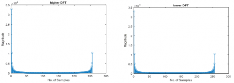
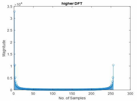
Figure 8 shows that when training and testing data are identical, the histogram and DFT seem very similar. Figure 9 shows the histogram shift and DFT magnitude when the number of training and testing samples is more than 12. In Figure 12a), the entire Modelsim simulation is shown. After the initial phase of training, the clock is applied and categorization begins. When the input data matches the learned data, the SOM-Hebb classifier returns the value 1. This is denoted in Matlab as "system matching with the trained data" in the window.
Figure 7. Framework of modelsim based TCM system
a) Histogram
b) DFT
Figure 8. Output waveform for same training and Test data
a) Histogram
b) DFT
Figure 9. Output waveform for unequal training and Test data
The accuracy of the TCM system is verified through experimentation. As was noted before, the method was designed to offer a sample clock synced to DFT computation so that the output text files are updated first in the learning mode. In the experiment, ModelSim was employed for pre-processing and keeping the trained data set ready. Further for each job, 256 samples were collected fora duration of 150sec. These data samples were acquired and written to the text documents. This process was repeated for 150 jobs. Obtained 30 datalog files, each of which contains 256 samples, were fed to a learning program executed on a PC as the training data. Table 3 represents the percentage error of the samples and the match and mismatch of the number of samples with respect to the nature of the job. DFT Magnitude for the lower range varies when the number of lower range samples is increased and vice versa for the higher range too. Figure 10 gives the histogram classification where lower and higher histogram represents the range of the samples which are having errors. The available training data from ModelSim were available in 32-D whose mean and median values with respect to job nature are represented in Figure 11. When the tool is under severe wear, the classifier output range changes and which itself results in the weak neuron, perturbation in spindle speed, feed rate, and depth of cut are not added during training. Perturbation was added during the process of data acquisition by changing spindle speed, and feed rate. The first test used training data without perturbation. The recognition rate was 96.4%.
Table 3. Nature of JOB and DFT computation
|
Test Number |
Number of low Level samples |
Number of samples within range |
Number of High level samples |
DFT Magnitude mean |
Nature of Job |
% Error |
|
|
Lower DFT |
Higher DFT |
||||||
|
Job 1 |
0 |
256 |
0 |
590.59 |
590.59 |
Normal |
0 |
|
Job 2 |
23 |
233 |
0 |
536.55 |
590.59 |
Severe Wear |
8.98 |
|
Job 3 |
0 |
256 |
0 |
590.59 |
590.59 |
Normal |
0 |
|
Job 4 |
0 |
256 |
0 |
590.59 |
590.59 |
Normal |
0 |
|
Job 5 |
0 |
256 |
0 |
590.59 |
590.59 |
Normal |
0 |
|
Job 6 |
0 |
256 |
0 |
590.59 |
590.59 |
Normal |
0 |
|
Job 7 |
0 |
256 |
0 |
590.59 |
590.59 |
Normal |
0 |
|
Job 8 |
0 |
256 |
0 |
590.59 |
590.59 |
Normal |
0 |
|
Job 9 |
0 |
256 |
0 |
590.59 |
590.59 |
Normal |
0 |
|
Job 10 |
0 |
256 |
0 |
590.59 |
590.59 |
Normal |
0 |
|
Job 11 |
0 |
256 |
0 |
590.59 |
590.59 |
Normal |
0 |
|
Job 12 |
0 |
179 |
77 |
590.59 |
411.58 |
Severe Wear |
30.07 |
|
Job 13 |
0 |
256 |
0 |
590.59 |
590.59 |
Normal |
0 |
|
Job 14 |
0 |
256 |
0 |
590.59 |
590.59 |
Normal |
0 |
|
Job 15 |
0 |
256 |
0 |
590.59 |
590.59 |
Normal |
0 |
|
Job 16 |
0 |
256 |
0 |
590.59 |
590.59 |
Normal |
0 |
|
Job 17 |
6 |
250 |
0 |
590.59 |
590.59 |
Partial wear |
2.34 |
|
Job 18 |
0 |
256 |
0 |
590.59 |
590.59 |
Normal |
0 |
|
Job 19 |
0 |
256 |
0 |
590.59 |
590.59 |
Normal |
0 |
|
Job 20 |
0 |
256 |
0 |
590.59 |
590.59 |
Normal |
0 |
|
Job 21 |
0 |
256 |
0 |
590.59 |
590.59 |
Normal |
0 |
|
Job 22 |
0 |
256 |
0 |
590.59 |
590.59 |
Normal |
0 |
|
Job 23 |
0 |
256 |
0 |
590.59 |
590.59 |
Normal |
0 |
|
Job 24 |
0 |
256 |
0 |
590.59 |
590.59 |
Normal |
0 |
|
Job 25 |
0 |
256 |
0 |
590.59 |
590.59 |
Normal |
0 |
|
Job 26 |
0 |
256 |
0 |
590.59 |
590.59 |
Normal |
0 |
|
Job 27 |
0 |
250 |
3 |
590.59 |
590.59 |
Partial wear |
1.17 |
|
Job 28 |
3 |
250 |
4 |
590.59 |
590.59 |
Partial wear |
2.73 |
|
Job 29 |
0 |
256 |
0 |
590.59 |
590.59 |
Normal |
0 |
|
Job 30 |
0 |
256 |
0 |
590.59 |
590.59 |
Normal |
0 |
Figure 10. Histogram and nature of job
Table 4. SOM-Hebb classifier recognition rate
|
SOM size |
Training |
Test |
Training |
Test |
Average |
|
A Data |
B Data |
B Data |
A Data |
||
|
16 × 16 |
96.4% |
97.92% |
97.16% |
||
Figure 11. SOM-Hebb classifier levels
Figure 12. Simulation results of a) output waveform of the classification using Modelsim b) Output of classification using Matlab
Presented a system of tool condition monitoring based on SOM and Hebb hybrid vector classifier. The suggested system's feature vector was time-invariant, and recognition was unaffected by changes in small input. The SOM-Hebb classifier was given a novel learning strategy in this research, where perturbed data is also verified. This method proposes a memoryless system which intern reduces the size and ultimately speed of the system. The whole recognition algorithm is implemented in HDL simulator Modelsim and tested its functionality. The system was designed to recognize vibration and temperature change and tested for 150 sets of data containing 256 samples each. The proposed systemcarries out classification at a speed of 256 samples/s with a recognition accuracy of 97.16% (Table 4).
The simulation results demonstrated that implementing a learning strategy can dramatically improve the system's recognition accuracy. The proposed strategy is easy to implement and very effective. The eventual goal is to synthesise such a system on FPGA and put it through its paces in terms of hardware performance and configurability testing. The reaction time and sliced area will be provided precisely by the hardware-implemented system. As on-chip learning is not currently included in simulation, it is proposed that it be implemented in the hardware in the following section. Users will be able to adaptively reinforce the system's learning against a specific data set that is known to induce false recognition thanks to on-chip learning. As a result, there is room to enhance precision.
[1] Sevilla-Camacho, P.Y., Robles-Ocampo, J.B., Jauregui-Correa, J.C., Jimenez-Villalobos, D. (2015). FPGA-based reconfigurable system for tool condition monitoring in high-speed machining process. Measurement, 64: 81-88. https://doi.org/10.1016/j.measurement.2014.12.037
[2] Mohanraj, T., Shankar, S., Rajasekar, R., Sakthivel, N. R., Pramanik, A. (2020). Tool condition monitoring techniques in milling process—A review. Journal of Materials Research and Technology, 9(1): 1032-1042. https://doi.org/10.1016/j.jmrt.2019.10.031
[3] Mohamed, A., Hassan, M., M’Saoubi, R., Attia, H. (2022). Tool condition monitoring for high-performance machining systems—A review. Sensors, 22(6): 2206. https://doi.org/10.3390/s22062206
[4] Hikawa, H., Kaida, K. (2014). Novel FPGA implementation of hand sign recognition system with SOM–Hebb classifier. IEEE Transactions on Circuits and Systems for Video Technology, 25(1): 153-166. https://doi.org/10.1109/TCSVT.2014.2335831
[5] Zhang, C., Zhang, J. (2013). On-line tool wear measurement for ball-end milling cutter based on machine vision. Computers in industry, 64(6): 708-719. https://doi.org/10.1016/j.compind.2013.03.010
[6] Atli, A.V., Urhan, O., Ertürk, S., Sönmez, M. (2006). A computer vision-based fast approach to drilling tool condition monitoring. Proceedings of the Institution of Mechanical Engineers, Part B: Journal of Engineering Manufacture, 220(9): 1409-1415. https://doi.org/10.1243/09544054JEM412
[7] Siddhpura, A., Paurobally, R. (2013). A review of flank wear prediction methods for tool condition monitoring in a turning process. The International Journal of Advanced Manufacturing Technology, 65: 371-393.https://doi.org/10.1007/s00170-012-4177-1
[8] Zhang, X.Y., Lu, X., Wang, S., Wang, W., Li, W.D. (2018). A multi-sensor based online tool condition monitoring system for milling process. Procedia CIRP, 72: 1136-1141. https://doi.org/10.1016/j.procir.2018.03.092
[9] Ambhore, N., Kamble, D., Chinchanikar, S., Wayal, V. (2015). Tool condition monitoring system: A review. Materials Today: Proceedings, 2(4-5): 3419-3428. https://doi.org/10.1016/j.matpr.2015.07.317
[10] Lazaro, J., Astarloa, A., Arias, J., Bidarte, U., Zuloaga, A. (2006). Simulink/Modelsim simulabel VHDL PID core for industrial SoPC multiaxis controllers. In IECON 2006-32nd Annual Conference on IEEE Industrial Electronics, pp. 3007-3011. https://doi.org/10.1109/IECON.2006.347606
[11] Cho, S., Asfour, S., Onar, A., Kaundinya, N. (2005). Tool breakage detection using support vector machine learning in a milling process. International Journal of Machine Tools and Manufacture, 45(3): 241-249. https://doi.org/10.1016/j.ijmachtools.2004.08.016
[12] MentorGraphics, "Modelsim". https://engineering.uiowa.edu/etc/help-desk-computer-services/software/mentor-graphics-modelsim.
[13] Ghosh, N., Ravi, Y.B., Patra, A., Mukhopadhyay, S., Paul, S., Mohanty, A.R., Chattopadhyay, A.B. (2007). Estimation of tool wear during CNC milling using neural network-based sensor fusion. Mechanical Systems and Signal Processing, 21(1): 466-479. https://doi.org/10.1016/j.ymssp.2005.10.010
[14] Cho, S., Binsaeid, S., Asfour, S. (2010). Design of multisensor fusion-based tool condition monitoring system in end milling. The International Journal of Advanced Manufacturing Technology, 46: 681-694. https://doi.org/10.1007/s00170-009-2110-z
[15] Franco-Gasca, L.A., de Jesús Romero-Troncoso, R., Herrera-Ruiz, G., del Rocío Peniche-Vera, R. (2009). FPGA based failure monitoring system for machining processes. The International Journal of Advanced Manufacturing Technology, 40: 676-686. https://doi.org/10.1007/s00170-008-1386-8
[16] Ohta, M., Kurosaki, Y., Ito, H., Hikawa, H. (2016). Effect of grouping in vector recognition system based on SOM. In 2016 IEEE Symposium Series on Computational Intelligence (SSCI), pp. 1-8. https://doi.org/10.1109/SSCI.2016.7850133
[17] Sridevi, K., Sundarambal, M., Dharan, K.M., Josephine, R.L. (2017). Hand gesture recognition system using radial basis function neural networks. Journal of Innovation in Electronics and Communication Engineering, 7(2): 38-41.
[18] Alex, A., L.L. (2016). Static hand sign recognition system with Som-Hebb classifier implemented in FPGA. International Journal of Engineering Science and Computing, pp. 2984-2987.
[19] Dai, Y., Zhu, K. (2018). A machine vision system for micro-milling tool condition monitoring. Precision Engineering, 52: 183-191.
[20] De Jesús, R.T.R., Gilberto, H.R., Iván, T.V., Carlos, J.C.J. (2004). FPGA based on-line tool breakage detection system for CNC milling machines. Mechatronics, 14(4): 439-454. https://doi.org/10.1016/S0957-4158(03)00069-2