Nguyen Hai Binh![]() | Vu Duy Hung*
| Vu Duy Hung*![]()
© 2023 IIETA. This article is published by IIETA and is licensed under the CC BY 4.0 license (http://creativecommons.org/licenses/by/4.0/).
OPEN ACCESS
The article introduces a bicyrobot built on the principle of gyroscope. A robust optimal controller has been designed to maintain a stable balance of the bicyrobot. However, the disadvantage of the controller is the high order. Therefore, the paper has applied Zhou's balanced truncation algorithm to reduce the order of high order controller. The results of order reduction of the high order controller show that the 3rd-order controller can replace the high order controller. The bicyrobot balance control system using a 3rd-order controller has the same quality as the bicyrobot balance control system using a high order controller.
robust controller, model order reduction algorithm, bicyrobot
Two-wheeled mobile robot has the advantage of flexibility and fast acceleration. However, the difficult problem of two-wheeled mobile robot is maintaining robot balance when the vehicle is stationary, when the vehicle is moving. Among the two-wheeled mobile robots, the bicyrobot is one of the robots that is of great interest to research [1-14].
There are many different solutions proposed to maintain balance for the bicyrobot, namely balance by moving the center of gravity [1-3], balance by centripetal force [4], balance by using a flywheel [5-14]. With the requirement that the robot needs to maintain balance even when stationary, the balancing method using the flywheel [5-14] has the best response, and this method also has a fast response. Therefore, it is appropriate to design bicyrobot balance control by flywheel method.
The balancing method using the flywheel is divided into two groups of methods.
The first method: using the flywheel according to the gyroscope principle [4-11].
The second method: using the flywheel according to the inverted pendulum principle [12-14].
The advantage of the first method is that it has a large balancing torque and high stability, but the disadvantage is that the energy consumed for the system is high.
The advantage of the second method is that the response of the system is fast, the energy consumption is low, but the balancing torque is not large.
To control bicyrobot, many algorithms have been proposed such as nonlinear algorithm [6], pole trajectory [7], PD algorithm [10], robust control algorithm [11-14], however, with the working environment of the two-wheeled mobile robot being an uncertain environment, the robust optimal control algorithm [11-14] is the most suitable for the two-wheeled mobile robot model. Robust optimal control theory is a modern control theory for designing optimal and stable controllers for control objects whose parameters change or are affected by external noise. However, the controller design according to the robust optimal control theory often obtains a high-order controller (the order of the controller is defined as the order of the sample polynomial). The high controller level has many disadvantages when we carry out the control on the robot, because the program code is complicated, the calculation time is long, so the response of the system will be slow. Therefore, reducing the model order [15-17] and reducing the controller order [11-14] while still ensuring the quality has a practical significance.
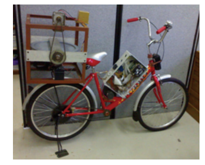
In the study [11], a bicyrobot model was built at Mechatronics Laboratory, Asian Institute of Technology (AIT) on a children's bicycle model. The vehicle model is designed to be able to go straight, reverse, and carry loads without falling down.
Figure 1. Bicyrobot model [11]
On the bicyrobot is arranged a flywheel, which is powered by a DC servo motor (Figure 1). The wheel always rotates at a fixed speed and will produce a constant torque. Use a DC motor to change the tilt angle of the flywheel along the Z axis (vertical axis from end to end of bicyrobot).
The principle of balance of the bicyrobot is as follows: When the bicyrobot deviates from the equilibrium position, the gravity of the bicyrobot will tend to pull the bicyrobot down. In order for the bicyrobot to be balanced, the control system will measure the tilt angle of the bicyrobot (q), then the control system will control the DC motor (change in motor input voltage–U) to change the tilt angle of the flywheel along the axis Z, the angular momentum in the Z axis produces a torque. This torque is called precession torque generated by gyroscope principle. The torque will balance with the torque generated by the bicyrobot's gravity, helping the bicyrobot return to the balanced position.
In the study [11], the authors modeled the bicyrobot in the unloaded state and obtained the following results:
$W(s)=\frac{\theta(\mathrm{s})}{\mathrm{U}(\mathrm{s})}=\frac{4887}{\mathrm{~s}^4+683.3 s^3+1208 s^2+109700 s-6949}$
in which, $\theta(\mathrm{s})$ the tilt angle of the bicyrobot; U(s) is DC motor input voltage. Details of the model building process and parameters of the bicyrobo model can be found in the study [11].
Bicyrobots in actual operation will be subject to many uncertainties such as changing loads, changing environmental conditions, so bicyrobots can be considered as uncertain models.
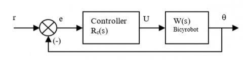
In the study [11], to control the balance of bicyrobots, the controller is designed according to the robust optimal control algorithm with the following control structure diagram (Figure 2).
Figure 2. Schematic diagram of the balance control structure bicyrobot [11]
where,
r - is reference tilt angle of bicyrobot
e(t) is tilt angle error of bicyrobot
U – is input voltage of DC motor
$\theta$ - is tilt angle of bicyrobot
Designing a bicyrobot balance controller according to a robust optimal control algorithm, the authors [11] obtained the following results:
$R_c(s)=\frac{A(s)}{B(s)}$
$\begin{align} & A\left( s \right)=1275{{s}^{5}}+{{8.695.10}^{5}}{{s}^{4}}+{{5.151.10}^{5}}{{s}^{3}} +{{1.359.10}^{8}}{{s}^{2}}+{{2.435.10}^{7}}s+{{1.091.10}^{6}} \\\end{align}$
$\begin{align} & B\left( s \right)={{s}^{6}}+715.7{{s}^{5}}+{{2.355.10}^{4}}{{s}^{4}}+{{2.789.10}^{5}}{{s}^{3}} +{{3.802.10}^{6}}{{s}^{2}}+{{6.519.10}^{5}}s+{{2.872.10}^{4}} \\\end{align}$
Zhou's balanced truncation algorithm [15, 16] is built on the basis of the balanced truncation algorithm [17]. The disadvantage of the balanced truncation algorithm [17] is that it only applies to stable linear systems. Zhou's balanced truncation algorithm can reduce order for both stable linear and unstable linear systems.
The content of Zhou's balanced truncation algorithm is as follows:
Input: Consider a linear, continuous, time-invariant parameter system with many inputs and many outputs, described in state space by the following system of equations:
$\begin{align} & \dot{x}=\mathbf{A}x+\mathbf{B}u \\ & y=\mathbf{C}x \\\end{align}$
in which, $x \in R^n, u \in R^p, y \in R^q, A \in R^{n x n}, B \in R^{n x p}, C \in R^{q x n}$. The order of the system is n.
Step 1. Determine the two matrices X and Y by solving the following system of equations:
$\begin{align} & \mathbf{XA}+\mathbf{A}'\mathbf{X}-\mathbf{XBB}'\mathbf{X}=0 \\ & \mathbf{AY}+\mathbf{YA}'-\mathbf{YC}'\mathbf{CY}=0 \\\end{align}$
Step 2. Let $F=-\boldsymbol{B}^{\prime} \boldsymbol{X}$ and $L=-\boldsymbol{Y} \boldsymbol{C}^{\prime}$
Step 3. Determine the control gramian matrix P and the observed gramian matrix Q by solving the following system of equations:
$\begin{align} & \left( \mathbf{A}+\mathbf{BF} \right)\mathbf{P}+\mathbf{P}\left( \mathbf{A}+\mathbf{BF} \right)'+\mathbf{BB}=0 \\ & \mathbf{Q}\left( \mathbf{A}+\mathbf{LC} \right)+\mathbf{A}\left( \mathbf{A}+\mathbf{LC} \right)'+\mathbf{C}'\mathbf{C}=0 \\\end{align}$
Step 4. Analyze the following matrices
Matrix Cholesky Analysis $\boldsymbol{P}=\boldsymbol{R R}^T$, with R is the upper triangular matrix.
Matrix SVD analysis $\boldsymbol{R} \boldsymbol{Q} \boldsymbol{R}^T=\boldsymbol{U} \boldsymbol{\Lambda} \boldsymbol{V}^T$.
Step 5. Calculate matrix $L=V^{1 / 2}$ .
Calculate non-degenerate matrix $(A, B, C)=\left(T^{-1} A T, T^{-1} B, C T\right)$.
Step 6. Calculate $(A, B, C)=\left(T^{-1} A T, T^{-1} B, C T\right)$.
Step 7. Choose r such that r < n, r is the order of the order reduction system.
The representation of (A,B,C) in block form is as follows:
$\mathbf{A}=\left[ \begin{matrix} {{\mathbf{A}}_{11}} & {{\mathbf{A}}_{12}} \\ {{\mathbf{A}}_{21}} & {{\mathbf{A}}_{22}} \\\end{matrix} \right]\text{, }\mathbf{B}=\left[ \begin{matrix} {{\mathbf{B}}_{1}} \\ {{\mathbf{B}}_{2}} \\\end{matrix} \right]\text{, }\mathbf{C}=\left[ \begin{matrix} {{\mathbf{C}}_{1}} & {{\mathbf{C}}_{2}} \\\end{matrix} \right],$
where, $\boldsymbol{A}_{11} \in R^{r x r}, \boldsymbol{B}_1 \in R^{r x p}, \boldsymbol{C}_1 \in R^{q x r}$.
Output: The order reduction system $\left(\boldsymbol{A}_{11}, \boldsymbol{B}_1, \boldsymbol{C}_1\right)$.
Performing order reduction of the 6th-order robust optimal controller according to Zhou's balanced truncation algorithm, the results are as follows:
Step 1. Matrix matrices X and Y:
$\mathbf{X}=\left[ \begin{align} & 0.0034\text{ }0.0157\text{ }0.0114\text{ }0.0079\text{ }0.0088\text{ }0.0078 \\ & 0.0157\text{ }0.0937\text{ }0.0688\text{ }0.0484\text{ }0.0530\text{ }0.0469 \\ & 0.0114\text{ }0.0688\text{ }0.0751\text{ }0.0601\text{ }0.0610\text{ }0.0538 \\ & 0.0079\text{ }0.0484\text{ }0.0601\text{ }0.1229\text{ }0.1226\text{ }0.1081 \\ & 0.0088\text{ }0.0530\text{ }0.0610\text{ }0.1226\text{ }0.6951\text{ }0.6205 \\& 0.0078\text{ }0.0469\text{ }0.0538\text{ }0.1081\text{ }0.6205\text{ }4.5791 \\\end{align} \right]$
$\mathbf{Y}=\left[ \begin{align} & \text{ 0}\text{.0021 -0}\text{.0023 -0}\text{.0167 0}\text{.0004 0}\text{.0030 0}\text{.0006} \\ & \text{-0}\text{.0023 0}\text{.0279 -0}\text{.0053 -0}\text{.1014 -0}\text{.0015 -0}\text{.0006} \\ & \text{-0}\text{.0167 -0}\text{.0053 0}\text{.4075 -0}\text{.0312 -0}\text{.0868 0}\text{.0032} \\ & \text{ 0}\text{.0004 -0}\text{.1014 -0}\text{.0312 0}\text{.6866 -0}\text{.2296 -0}\text{.4141} \\ & \text{ 0}\text{.0030 -0}\text{.0015 -0}\text{.0868 -0}\text{.2296 3}\text{.4409 -1}\text{.9749} \\ & \text{ 0}\text{.0006 -0}\text{.0006 0}\text{.0032 -0}\text{.4141 -1}\text{.9749 37}\text{.8832} \\\end{align} \right]$
Step 2. The matrices F and L are defined as follows:
$\mathbf{F}=\left[ -0.4320\text{ -}2.0086\text{ }-1.4645\text{ }-1.0151\text{ }-1.1252\text{ }-0.9966 \right]$
$\mathbf{L}=\left[ \begin{matrix} \text{9}\text{.0849} & 0 & 0 & 0 & 0 & 0 \\ 0 & \text{2}\text{.4594} & 0 & 0 & 0 & 0 \\ 0 & 0 & \text{1}\text{.5076} & 0 & 0 & 0 \\ 0 & 0 & 0 & \text{0}\text{.0179} & 0 & 0 \\ 0 & 0 & 0 & 0 & \text{0}\text{.0002} & 0 \\ 0 & 0 & 0 & 0 & 0 & 0 \\\end{matrix} \right]$
Step 3. The control gramian matrix P and the observed gramian matrix Q are as follows:
$\mathbf{P}=\left[ \begin{align} & \text{11}\text{.1786 0}\text{.0000 -1}\text{.9446 -0}\text{.0000 0}\text{.0280 0}\text{.0000} \\ & \text{ 0}\text{.0000 3}\text{.8892 -0}\text{.0000 -1}\text{.7926 0}\text{.0000 0}\text{.0024} \\ & \text{-1}\text{.9446 -0}\text{.0000 7}\text{.1704 0}\text{.0000 -0}\text{.6071 0}\text{.0000} \\ & \text{-0}\text{.0000 -1}\text{.7926 0}\text{.0000 4}\text{.8565 -0}\text{.0000 -0}\text{.0963} \\& \text{ 0}\text{.0280 0}\text{.0000 -0}\text{.6071 -0}\text{.0000 0}\text{.7702 -0}\text{.0000} \\ & \text{ 0}\text{.0000 0}\text{.0024 0}\text{.0000 -0}\text{.0963 -0}\text{.0000 0}\text{.1114} \\\end{align} \right]$
$\mathbf{Q}=\left[ \begin{align} & \text{0}\text{.7539 4}\text{.0166 0}\text{.0303 0}\text{.6022 0}\text{.0546 0}\text{.0099} \\ & \text{4}\text{.0166 21}\text{.4076 0}\text{.2402 3}\text{.2096 0}\text{.2910 0}\text{.0528} \\ & \text{0}\text{.0303 0}\text{.2402 0}\text{.8415 0}\text{.0469 0}\text{.0035 0}\text{.0006} \\ & \text{0}\text{.6022 3}\text{.2096 0}\text{.0469 0}\text{.9802 0}\text{.0892 0}\text{.0162} \\ & \text{0}\text{.0546 0}\text{.2910 0}\text{.0035 0}\text{.0892 0}\text{.0086 0}\text{.0016} \\ & \text{0}\text{.0099 0}\text{.0528 0}\text{.0006 0}\text{.0162 0}\text{.0016 0}\text{.0003} \\\end{align} \right]$
Step 4 - Step 5. The transition matrix T has the following form:
$\mathbf{T}=\left[ \begin{align} & \text{-0}\text{.2878 -1}\text{.5333 -0}\text{.0114 -0}\text{.2197 -0}\text{.0199 -0}\text{.0036} \\ & \text{ 0}\text{.0002 -0}\text{.0540 -0}\text{.5844 -0}\text{.0083 -0}\text{.0002 -0}\text{.0000} \\ & \text{-0}\text{.0309 -0}\text{.1644 -0}\text{.0135 -0}\text{.5994 -0}\text{.0547 -0}\text{.0100} \\ & \text{ 0}\text{.0001 -0}\text{.0007 -0}\text{.0132 0}\text{.0008 -0}\text{.1564 -0}\text{.0565} \\ & \text{-0}\text{.0036 0}\text{.0022 -0}\text{.0011 0}\text{.0008 -0}\text{.0007 -0}\text{.0003} \\ & \text{-0}\text{.0000 0}\text{.0000 -0}\text{.0000 0}\text{.0000 -0}\text{.0000 0}\text{.0002} \\\end{align} \right]$
Step 6. The system is in equilibrium:
$\mathbf{A}=\left[ \begin{align} & \text{-33}\text{.5488 -10}\text{.0630 -1}\text{.4287 0}\text{.1713 -1}\text{.3186 0}\text{.0001} \\ & \text{ 25}\text{.4119 -0}\text{.0475 -9}\text{.3031 0}\text{.0212 -0}\text{.1632 0}\text{.0000} \\ & \text{ -3}\text{.6407 14}\text{.6874 -0}\text{.1800 0}\text{.0257 -0}\text{.2272 0}\text{.0000} \\ & \text{ 0}\text{.5301 -0}\text{.0330 0}\text{.3351 -0}\text{.0995 1}\text{.4997 -0}\text{.0001} \\ & \text{ -1}\text{.3457 1}\text{.0529 -0}\text{.6188 3}\text{.4541 -681}\text{.7340 0}\text{.0833} \\ & \text{ -0}\text{.0001 0}\text{.0000 -0}\text{.0001 0}\text{.0001 -0}\text{.0948 -0}\text{.0902} \\\end{align} \right]$
$\mathbf{B}=\left[ \begin{align} & \text{-36}\text{.8367} \\ & \text{0}\text{.0209} \\ & \text{-3}\text{.9522} \\ & \text{0}\text{.0140} \\ & \text{-0}\text{.4623} \\ & \text{-0}\text{.0000} \\\end{align} \right]$
$\mathbf{C}=\left[ \text{-34}\text{.5138 -0}\text{.1458 -0}\text{.8641 0}\text{.0590 -0}\text{.4592 0}\text{.0000} \right]$
Step 7. The results of order reduction of the 6th order robust optimal controller are shown in Table 1 as follows:
Table 1. The results of order reduction of the 6th-order robust optimal controller
|
Order |
Rr(s) |
$\left\|\mathbf{R}-\mathbf{R}_{\mathbf{r}}\right\|_{\infty}$ |
|
4 |
$\frac{1275 s^3+356.8 s^2+1.993 .10^5 s+1.922 .10^4}{s^4+33.88 s^3+398.1 s^2+5544 s+507}$ |
0.0702 |
|
3 |
$\frac{1275 s^2+231.2 s+1.993 .10^5}{s^3+33.78 s^2+394.8 s+5504}$ |
1.7868 |
|
2 |
$\frac{1271 s+204}{s^2+33.6 s+257.3}$ |
37.1945 |
|
1 |
$\frac{1271}{s+33.55}$ |
37.9080 |
Figure 3. Step response of the 4th-order robust optimal controller, the 3rd- order robust optimal controller and the 6th-order robust optimal controller
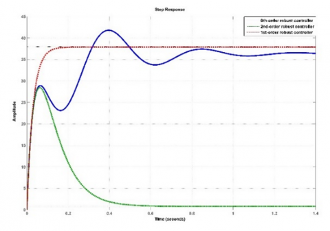
To evaluate the low-order robust optimal controllers, using Matlab-Simulink software we compare the step response and bode response of the low-order robust optimal controllers with the original controller, the results are shown in Figure 3-Figure 6 as follows.
According to the results in Figure 3: The step response of the 4th-order robust optimal controller, the 3rd-order robust optimal controller completely coincides with the step response of the 6th-order robust optimal controller.
Figure 4. Step response of the 4th-order robust optimal controller, the 3rd- order robust optimal controller and the 6th-order robust optimal controller
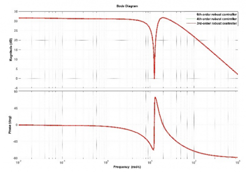
Figure 5. Bode response of the 4th-order robust optimal controller, the 3rd- order robust optimal controller and the 6th-order robust optimal controller
According to the results in Figure 4: Step response of the 2nd-order robust optimal controller, the 1st- order robust optimal controller has a large deviation from the step response of the 6th-order robust optimal controller.
According to the results in Figure 5: The bode response of the 4th-order robust optimal controller, the 3rd-order robust optimal controller completely coincides with the step response of the 6th-order robust optimal controller.
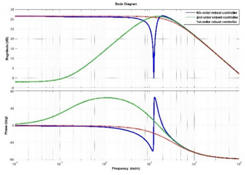
According to the results in Figure 6: Bode response of the 2nd-order robust optimal controller, the 1st- order robust optimal controller and the 6th-order robust optimal controller.
In the frequency range w> 30.5 rad/s, the frequency response of the 2nd-order robust optimal controller coincides with that of the 6th-order robust optimal controller.
In the frequency range w < 30.5 rad/s, the frequency response of the 2nd-order robust optimal controller deviates from the 6th-order robust optimal controller's frequency response.
Figure 6. Bode response of the 2nd-order robust optimal controller, the 1st- order robust optimal controller and the 6th-order robust optimal controller
In the frequency range w < 0.0752 rad/s and w > 89.7 rad/s, the frequency response of the 1st-order robust optimal controller coincides with that of the 6th-order robust controller.
In the frequency range 0,0752 rad/s< w < 89,7 rad/s, the frequency response of the 1nST-order robust optimal controller deviates from the 6th-order robust optimal controller's frequency response.
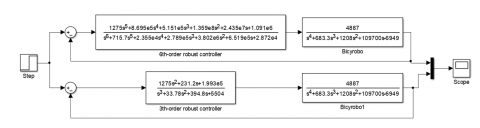
Simulink diagram of the bicyrobot balance control system using a robust 3rd-order robust optimal controller and a 6th-order robust optimal controller is shown in the following Figure 7.
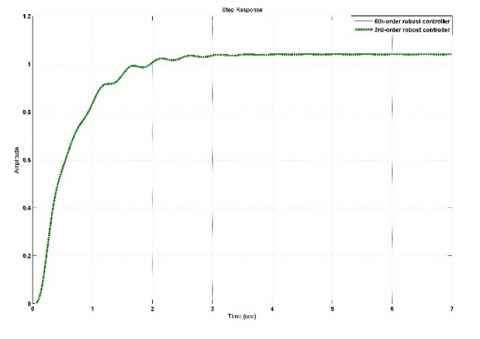
The response result of the bicyrobot balance control system when using the 3rd-order robust optimal controller and when using the 6th-order robust optimal controller is shown in the following Figure 8.
According to the results in Figure 8: The step response of the bicyrobot control system using a 3rd-order robust optimal controller completely coincides with the step response of the bicyrobot control system using a 6th-order robust optimal controller.
Simulink diagram of the bicyrobot balance control system using a robust 1st-order robust optimal controller and a 6th-order robust optimal controller is shown in the following Figure 9.
Figure 7. Simulink diagram simulating a bicyrobot balance control system using a robust 3rd-order robust optimal controller and a 6th-order robust optimal controller
Figure 8. The step response of the bicyrobot balance control system when using the 3rd-order robust optimal controller and when using the 6th-order robust optimal controller
Figure 9. Simulink diagram simulating a bicyrobot balance control system using a robust 1st-order robust optimal controller and a 6th-order robust optimal controller
The response result of the bicyrobot balance control system when using the 1st-order robust optimal controller and when using the 6th-order robust optimal controller is shown in the following Figure 10.
According to the results in Figure 10, the bicyrobot balance control system using 1st-order robust optimal controller does not guarantee stable balancing of the bicyrobot.
Figure 10. The step response of the bicyrobot balance control system when using the 1st-order robust optimal controller and when using the 6th-order robust optimal controller
Design a bicyrobot balance controller according to the robust optimal control algorithm to obtain a 6th-order robust optimal controller. The 6th-order robust optimal controller when applying the real control of the bicyrobot balancing system will face many disadvantages, so it is necessary to reduce the order of this controller. The 6th-order robust optimal controller is a stable linear system. Zhou's balanced truncation algorithm can be applied to reduce the order of both stable and unstable linear systems. Applying Zhou's balanced truncation algorithm to reduce the order of the 6th-order robust optimal controller will hel9p to obtain order reduction systems with small errors. Using low-order robust optimal controllers to control the balance of the bicyrobot shows that: The step response of the system when using the 3rd-order robust optimal controller completely coincides with the step response of the system when using the 6th-order robust optimal controller. The 1st-order robust optimal controller cannot control the balance of the bicyrobot. The 3rd-order robust optimal controller is the most suitable controller to replace the 6th-order robust optimal controller. The simulation results show the correctness of Zhou's balanced truncation algorithm and the robust optimal control algorithm.
The authors gratefully acknowledge the University of Economics–Technology for Industries for supporting this work.
[1] Keo, L., Yoshino, K., Kawaguchi, M., Yamakita, M. (2011). Experimental results for stabilizing of a bicycle with a flywheel balancer. In 2011 IEEE International Conference on Robotics and Automation, pp. 6150-6155. https://doi.org/10.1109/ICRA.2011.5979991
[2] Chen, C.K., Dao, T.K. (2010). Speed-adaptive roll-angle-tracking control of an unmanned bicycle using fuzzy logic. Vehicle System Dynamics, 48(1): 133-147. https://doi.org/10.1080/00423110903085872
[3] Huang, C.F., Tung, Y.C., Yeh, T.J. (2017). Balancing control of a robot bicycle with uncertain center of gravity. In 2017 IEEE International Conference on Robotics and Automation (ICRA), pp. 5858-5863. https://doi.org/10.1109/ICRA.2017.7989689
[4] Lee, S., Ham, W. (2002). Self stabilizing strategy in tracking control of unmanned electric bicycle with mass balance. In IEEE/RSJ International Conference on Intelligent Robots And Systems, 3: pp. 2200-2205. https://doi.org/10.1109/IRDS.2002.1041594
[5] Keo, L., Yoshino, K., Kawaguchi, M., Yamakita, M. (2011). Experimental results for stabilizing of a bicycle with a flywheel balancer. In 2011 IEEE International Conference on Robotics and Automation, pp. 6150-6155. https://doi.org/10.1109/ICRA.2011.5979991
[6] Beznos, A.V., Formal'Sky, A.M., Gurfinkel, E.V., Jicharev, D.N., Lensky, A.V., Savitsky, K.V., Tchesalin, L.S. (1998). Control of autonomous motion of two-wheel bicycle with gyroscopic stabilisation. In Proceedings. 1998 IEEE International Conference on Robotics and Automation (Cat. No. 98CH36146), 3: pp. 2670-2675. https://doi.org/10.1109/ROBOT.1998.680749
[7] Yetkin, H., Kalouche, S., Vernier, M., Colvin, G., Redmill, K., Ozguner, U. (2014). Gyroscopic stabilization of an unmanned bicycle. In 2014 American Control Conference, pp. 4549-4554. https://doi.org/10.1109/ACC.2014.6859392
[8] Lam, P.Y. (2011). Gyroscopic stabilization of a kid-size bicycle. In 2011 IEEE 5th International Conference on Cybernetics and Intelligent Systems (CIS), pp. 247-252. https://doi.org/10.1109/ICCIS.2011.6070336
[9] Hwang, S.I., Ha, H.M., Lee, J.M. (2015). Balancing and driving control of a mecanum wheel ball robot. Journal of Institute of Control, Robotics and Systems, 21(4): 336-341. https://doi.org/10.5302/J.ICROS.2015.14.0127
[10] Suprapto, S. (2006). Development of a gyroscopic unmanned bicycle. M. Eng. Thesis, Asian Institute of Technology, Thailand.
[11] Thanh, B.T., Parnichkun, M. (2008). Balancing control of bicyrobo by particle swarm optimization-based structure-specified mixed H2/H∞ control. International Journal of Advanced Robotic Systems, 5(4): 39. https://doi.org/10.5772/6235
[12] Vu, N.K., Nguyen, H.Q. (2020). Balancing Control of Two-Wheel Bicycle Problems. Mathematical Problems in Engineering, 2020: Article ID 6724382. https://doi.org/10.1155/2020/6724382
[13] Kien, V.N., Quang, N.H., Trung, N.K. (2021). Application of model reduction for robust control of self-balancing two-wheeled bicycle. TELKOMNIKA (Telecommunication Computing Electronics and Control), 19(1): 252-264. http://doi.org/10.12928/telkomnika.v19i1.16298
[14] Vu, N.K., Nguyen, H.Q. (2021). Design low-order robust controller for self-balancing two-wheel vehicle. Mathematical problems in engineering, 2021: Article ID 6693807. https://doi.org/10.1155/2021/6693807
[15] Zhou, K., Salomon, G., Wu, E. (1999). Balanced realization and model reduction for unstable systems. International Journal of Robust and Nonlinear Control: IFAC‐Affiliated Journal, 9(3): 183-198. https://doi.org/10.1002/(SICI)1099-1239(199903)9:3%3C183::AID-RNC399%3E3.0.CO;2-E
[16] Vu, N.K., Nguyen, H.Q. (2021). Model reduction of unstable systems based on balanced truncation algorithm. International Journal of Electrical & Computer Engineering, 11(3): 2045-2053. http://doi.org/10.11591/ijece.v11i3.pp2045-2053
[17] Moor, B.C. (1981). Principle component analysis in linear system. IEEE Trans Autom Control, 11: 17-32. https://doi.org/10.1109/TAC.1981.1102568