Mercy Rosalina Kotapuri* | Rajesh Kumar Samala
© 2021 IIETA. This article is published by IIETA and is licensed under the CC BY 4.0 license (http://creativecommons.org/licenses/by/4.0/).
OPEN ACCESS
The idea about this proposed work, to know the Distributed Generation (DG) impact on distribution scheme. This is to improve the performance of the system using power loss reduction and voltage development. In this proposed work Wind Turbine (WT) and Photo-Voltaic (PV) units were taken for DGs and various algorithms are tested to get the effect of DG on network. In this paper one new hybrid algorithm is proposed to have optimal size and location of various types of DGs. Initially, active and reactive power losses of the test system and voltage at every bus of the test system were examined using Back and Forward (B/FW) Sweep technique. Similarly, Gravitational Search Analysis (GSA), BAT Analysis (BA) and Ant Lion Optimization (ALO) techniques were utilized to examine the parameters of the same test system. Finally, all the constraints were compared with projected hybrid approach. All the algorithms have tested on IEEE-33 and IEEE-69 standard test systems. Furthermore, the MATLAB simulation is used to get the optimal allocation of DGs.
distributed generation, gravitational search analysis, BAT analysis, ant-lion optimization, power loss, optimal location, capacity
The world wide apprehensions about the atmosphere, associated along with development of techniques to link non-conventional energy resources to grid and electric power market deregulation of has abstracted the distribution planners concentration towards distributed generation (DG) connection to grid-connected [1, 2]. DG known as a small-scale electrical energy generation for the requirement of sustaining station load dissimilar from the conventional or Central power station [3]. Majority of DG sources are considered with the help of green energy that is assumed pollution free. Penetration of have many technical advantages.
Furthermore, DG is accessible in modular unit, considered by easy of identify location for small generators, little construction times, and minimum capital investment [4, 5]. The technical advantages of DG include improvement of voltage, reduction in loss of power, relieved from transmission and distribution congestion, enhanced network reliability and quality of power. All the above are aids to accomplished by introducing DGs at correct sites with correct capacity otherwise, it could lead to adverse effects like augmented power losses [6, 7]. The wrong placement will leads to raise in scheme losses and sometimes it may even collapse the entire scheme [8]. Though, the tasks of detecting the optimal sizes and sites of DG units in distribution scheme are not easy [9].
Now the DG installation is placing a big vital role in distribution schemes due to its advantages over the methods in reduction in network total power loss, reduction in total operating power of the network, user friendly and environmental friendly, increase in system voltage, and reliability [10, 11]. The placement of DG is purely the choice of its owners and also investors. It also depends on location and the availability of the fuel and condition of climate [12, 13]. Though the introduction and the modifications depend on number of DGs installation like one or single DG installation and installation of multi-DGs. Various techniques have presented to find the optimal site and capacity of the DG [14-17]. Besides the reduction in power loss, the DG location is may be on the basis of reduction in cost. The mixed integer linear program, Tabu Search (TS), Genetic Approach (GA), Particle Swarm Optimization (PSO) approach, Ant Colony Optimization (ACO) and direct search approach are utilized to calculate the best DG location and siting. In those papers when introducing DGs emphasis is provided on the reduction in line loss [18-20]. Consequently, the optimization approaches would be engaged for deregulation of power industry, permitting for the optimal allocation of the DG. In the work, an efficient approach is projected to validate the load flow issue and the placement issue of DG.
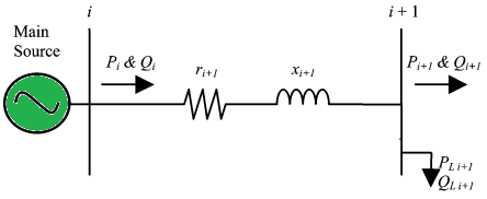
Figure 1 represents a simple two bus system. This work is to examine the suitable size and site of DG. The main objective in this research is enhancement of voltage and minimization of power losses.
Figure 1. Single line layout of two bus scheme
$VoltageDeviationIndex=\sum\limits_{i}^{N}{\frac{\left| {{V}_{rated-{{V}_{i}}}} \right|}{{{V}_{rated}}}}$ (1)
where, Vrated be the network rated value of voltage and it is 1.0 p.u. Vi be the ith bus voltage in p.u. N be the network total buses number.
Minimization of real power loss $=\left(\begin{array}{l}N_{b u s} \\ \sum_{i=2}\left(P_{g n i}-P_{d n i}-V_{m i} V_{n i} Y_{m n i} \cos \left(\delta_{m i}-\delta_{n i}+\theta_{n i}\right)\right)\end{array}\right)$ (2)
where, Pgni is generator output active power at bus ni, Pdni is the active power demand at bus ni, Vmi be the voltage of bus mi, Vni be the voltage of bus ni, Ymni be the admittance magnitude among mi bus and bus ni, δmi be the voltage phase angle at bus mi, δni be the voltage phase angle at bus ni, θni be the angle of admittance of Yi=Yni∟θni. Nbus represents number of buses in given test scheme, Ni is receiving bus number (Ni = 2, 3, Nn) and mi is the bus number that sending power to bus ni (m2 = n1 = 1) and i is the branch number that fed bus ni.
2.1 Constraints
$\begin{align} & {{P}_{Gi}}-{{P}_{Di}}-{{V}_{i}}\left( \sum\limits_{j=1}^{{{N}_{bus}}}{\left( {{V}_{j}} {{Y}_{ij}} cos({{\delta }_{j}}-{{\delta }_{i}}+{{\theta }_{ij}}) \right)} \right)=0 \\ & {{Q}_{Gi}}-{{Q}_{Di}}-{{V}_{i}}\left( \sum\limits_{j=1}^{{{N}_{bus}}}{\left( {{V}_{j}} {{Y}_{ij}} sin({{\delta }_{j}}-{{\delta }_{i}}+{{\theta }_{ij}}) \right)} \right)=0 \\ & i = 1, 2, ...., Nbus \\\end{align}$ (3)
Here PGiand QGistates active and reactive power generated at i bus respectively; PDiand QDistates active and reactive load at i bus respectively, Piand Qistates active and reactive injected power at i bus, Yijand θijstates the amplitude of admittance and branch voltage angle connecting i and j buses.
2.1.1 Voltage limits
For this paper work, the deviation of voltage is definite from 1.05 pu and 0.90 pu.
${{V}_{\max }}\ge V\ge {{V}_{\min }}$ (4)
Here: Vmax be the peak voltage of bus and Vmin be the lowest voltage of bus.
2.1.2 Real power loss constraint
$P{{L}_{withoutDG}}\ge P{{L}_{withDG}}$ (5)
2.1.3 DG constraint
$\sum\limits_{i=1}^{Nbus}{{}}{{P}_{Di}}\ge {{P}_{DG}}\ge {{0}_{{}}}$ (6)
$\sum\limits_{i=1}^{Nbus}{{}}{{Q}_{Di}}\ge {{Q}_{DG}}\ge {{0}_{{}}}$ (7)
where, PDiand QDiare the active and reactive load demand at the same bus.
Algorithm:
${{V}_{i}}={{V}_{i+1}}+conj(({{P}_{i+1}}+j{{Q}_{i+1}})/{{V}_{i+1}})$ (8)
${{P}_{i}}={{P}_{i\_Load}}+{{P}_{i\_Loss}}$ (9)
${{Q}_{i}}={{Q}_{i\_Load}}+{{Q}_{i\_Loss}}$ (10)
${{P}_{i\_Loss}}={{(({{P}_{i+1}}^{2}+{{Q}_{i+1}}^{2})/{{V}_{i+1}}^{2})}^{{}}}*{{R}_{i}}^{{}}$ (11)
${{Q}_{i\_Loss}}={{(({{P}_{i+1}}^{2}+{{Q}_{i+1}}^{2})/{{V}_{i+1}}^{2})}^{{}}}*{{X}_{i}}^{{}}$ (12)
where, Vi is the node current voltage, Vi+1 is voltage at next node, Pi+1 is next node active power, Qi+1 is next node reactive power, Ri is the line resistance among i and i+1 node and Xi is the line reactance line among i and i+1 node.
${{\varepsilon }_{{}}}\ge {{V}_{calculated}}-{{V}_{described}}$ (13)
Here ε specified the tolerance.
${{V}_{i+1}}={{V}_{i}}+conj(({{P}_{i}}+j{{Q}_{i}})/{{V}_{i}})$ (14)
${{P}_{i}}={{P}_{i\_Load}}+{{P}_{i\_Loss}}$ (15)
${{Q}_{i}}={{Q}_{i\_Load}}+{{Q}_{i\_Loss}}$ (16)
${{P}_{i\_Loss}}={{(({{P}_{i}}^{2}+{{Q}_{i}}^{2})/{{V}_{i}}^{2})}^{{}}}*{{R}_{i}}^{{}}$ (17)
${{Q}_{i\_Loss}}={{(({{P}_{i}}^{2}+{{Q}_{i}}^{2})/{{V}_{i}}^{2})}^{{}}}*{{X}_{i}}^{{}}$ (18)
DGs were considering as generator buses and load buses in the case of power flow studies. The DG should reach their reacive power constraint when DG is considered as generator bus and finally this generator bus converts into load bus.
In this case, DG generates fixed real power and reactive power [21]. Hence, real power load and reactive power load at the interconnected bus (PL and QL) are changed as given in Eqns. (19) and (20),
${{P}_{L}}(t)={{P}_{L}}(t)-{{P}_{DG}}(t)$ (19)
${{Q}_{L}}(t)={{Q}_{L}}(t)-{{Q}_{DG}}(t)$ (20)
Now, this multi-objective function is for reduction in real power losses and voltage improvement at all buses. Classification of DG sources as 4 – types [22].
Type1: Active power injecting only.
Type2: Reactive power injecting only
Type3: Injecting both powers active and reactive.
Type4: Injecting active but consuming reactive power.
The projected methodology is an effective method for getting the finest capacity and site the DG. This supirior methodology is a hybridization of BA and ALO to improve the outcome of the test scheme. The ALO approach is employed to estimation of loss of real power. The outcome of the ALO approach is having high iteration to achieve the better outcome and poor performance. To enhance the performance of ALO which is based on the BAT approaach. The process of the projected technique is presented in subsequent section and the flow chart for the proposed method is shown in Figure 2.
Figure 2. Proposed hybrid technique flow chart
This projected scheme is worked on MATLAB. Outcome is tested on IEEE-33 which have of 33 buses and 32 branches with 12.66 kV and 100 MVA are base values and 3.715 MW is complete real and 2.3 MVAR is complete reactive power load shown in Figure 3 and IEEE-69 which have of 69 buses and 68 branches with 12.66 kV and 100 MVA are base values and 3.80219 MW is complete real and 2.6946 MVAR is total reactive power load shown in Figure 4, Power factor of this scheme is 0.85 lagging, 0.85 leading and Unity. For the implementation purpose, projected hybridization technique and traditional scheme parameters are given in Table 1.
Figure 3. IEEE-33 standard test system
Figure 4. IEEE-69 test bus
Table 1. Implementation parameters
|
Description |
Algorithms |
Values |
|
Population size (n) |
BA |
20 |
|
Number of generations (N) |
10 |
|
|
Loudness (A) |
1 |
|
|
Pulse rate (r) |
1 |
|
|
Frequency (Q) |
(0,2) |
|
|
Dimension (d) |
4 |
|
|
Ant lion pits |
ALO |
3 |
|
Number of Ant lions |
10 |
|
|
Max iteration |
100 |
In this paper, two DGs has considered for better site and sized. All the objecctives like DG capacity, DG site, loss of active power, cost of power loss, cost of DGs and Voltage Stability Index (VSI) when the power factor is unity, 085 lagging and 0.85 leading using various methods of algorithms are reported in Tables 2 to 5. In Table 6 comparison analysis of power loss and VSI are mentioned. In Table 7 & 8 cost of Power Loss validation per year for IEEE-33 and IEEE-69 bus scheme has done. In Tables 9 & 10 cost of DG validationn per annum for IEEE-33 bus and IEEE-69 bus scheme has done.
Table 2. Optimal location and capacity of DG using GSA method on IEEE-33 & 69 Bus
|
Bus No |
Normal Power Loss (kW) |
Power loss (kW) |
% Reduction |
DG capacity (kW) |
Optimal bus connected for DG |
Load connected Bus |
|||
|
Load Power Loss |
GSA Power Loss |
||||||||
|
PV |
WT |
PV |
WT |
||||||
|
33 |
210.016 |
220.7793 |
207.6548 |
5.94 |
12 |
204 |
4 |
19 |
24 |
|
225.8542 |
200.4888 |
11.23 |
85 |
190 |
2 |
27 |
31 |
||
|
223.8893 |
198.9805 |
11.12 |
100 |
196 |
22 |
6 |
29 |
||
|
220.0239 |
201.2303 |
8.54 |
60 |
193 |
3 |
4 |
7 |
||
|
69 |
237.9656 |
241.4972 |
226.566 |
6.18 |
12 |
205 |
20 |
20 |
10 |
|
238.2408 |
232.6279 |
2.35 |
85 |
160 |
48 |
24 |
48 |
||
|
386.3267 |
230.712 |
40.28 |
100 |
153 |
12 |
30 |
60 |
||
|
261.2378 |
227.2329 |
13.01 |
60 |
165 |
12 |
14 |
63 |
||
Table 3. Optimal location and capacity of DG using BAT method on IEEE-33 & 69 Bus
|
Bus No |
Normal Power Loss (kW) |
Power loss (kW) |
% Reduction |
DG capacity (kW) |
Optimal bus connected for DG |
Load connected Bus |
|||
|
Load Power Loss |
BAT Power Loss |
||||||||
|
PV |
WT |
PV |
WT |
||||||
|
33 |
210.016 |
220.7793 |
206.5204 |
6.45 |
12 |
160 |
20 |
14 |
24 |
|
225.8542 |
172.3606 |
23.68 |
85 |
190 |
16 |
16 |
31 |
||
|
223.8893 |
170.8101 |
23.70 |
100 |
179 |
18 |
31 |
29 |
||
|
220.0239 |
180.0811 |
18.15 |
60 |
172 |
10 |
17 |
7 |
||
|
69 |
237.9656 |
241.4972 |
226.7515 |
6.10 |
12 |
209 |
24 |
26 |
10 |
|
238.2408 |
224.9875 |
5.56 |
85 |
158 |
54 |
19 |
48 |
||
|
386.3267 |
224.867 |
41.79 |
100 |
196 |
53 |
68 |
60 |
||
|
261.2378 |
193.4544 |
25.94 |
60 |
204 |
61 |
58 |
63 |
||
Table 4. Optimal location and capacity of DG using ALO method on IEEE-33 & 69 Bus
|
Bus No |
Normal Power Loss (kW) |
Power loss (kW) |
% Reduction |
DG capacity (kW) |
Optimal bus connected for DG |
Load connected Bus |
|||
|
Load Power Loss |
ALO Power Loss |
||||||||
|
PV |
WT |
PV |
WT |
||||||
|
33 |
210.016 |
220.7793 |
183.806 |
16.74 |
12 |
163 |
18 |
17 |
24 |
|
225.8542 |
177.209 |
21.53 |
85 |
156 |
16 |
11 |
31 |
||
|
223.8893 |
150.4867 |
32.78 |
100 |
198 |
12 |
18 |
29 |
||
|
220.0239 |
183.7687 |
16.47 |
60 |
169 |
9 |
11 |
7 |
||
|
69 |
237.9656 |
241.4972 |
236.312 |
2.14 |
12 |
178 |
45 |
58 |
10 |
|
238.2408 |
187.3165 |
21.37 |
85 |
217 |
62 |
59 |
48 |
||
|
386.3267 |
212.3519 |
45.03 |
100 |
216 |
8 |
60 |
60 |
||
|
261.2378 |
218.3531 |
16.41 |
60 |
196 |
20 |
60 |
63 |
||
Table 5. Optimal location and capacity of DG using proposed method on IEEE-33 & 69 Bus
|
Bus No |
Normal Power Loss (kW) |
Power loss (kW) |
% Reduction |
DG capacity (kW) |
Optimal bus connected for DG |
Load connected Bus |
|||
|
Load Power Loss |
Proposed Power Loss |
||||||||
|
PV |
WT |
PV |
WT |
||||||
|
33 |
210.016 |
220.7793 |
173.856 |
21.25 |
12 |
153 |
18 |
7 |
2 |
|
225.8542 |
167.009 |
26.05 |
85 |
150 |
16 |
15 |
12 |
||
|
223.8893 |
138.2429 |
38.25 |
100 |
135 |
12 |
10 |
14 |
||
|
220.0239 |
156.4589 |
28.89 |
60 |
162 |
19 |
25 |
25 |
||
|
69 |
237.9656 |
241.4972 |
216.256 |
10.45 |
12 |
158 |
40 |
55 |
6 |
|
238.2408 |
166.8459 |
29.96 |
85 |
207 |
60 |
59 |
9 |
||
|
386.3267 |
155.4853 |
59.75 |
100 |
166 |
18 |
62 |
52 |
||
|
261.2378 |
202.6521 |
22.42 |
60 |
176 |
25 |
60 |
63 |
||
Table 6. Comparison analysis of power loss and VSI
|
Methods |
Power Loss (kW) |
VSI (p.u) |
|
Proposed Method |
138.25 |
0.64451 |
|
ALO |
150.55 |
0.9847 |
|
BAT |
180.57 |
0.9578 |
|
GSA[24] method |
182.19 |
0.9364 |
|
IWD[23] |
185.78 |
0.9155 |
|
BFOA [23] |
186.48 |
0.9047 |
|
Multi objective particle swarm optimization (MOPSO) [23] |
194.25 |
0.87 |
|
Particle Swarm Optimization (PSO) [23] |
204.78 |
0.81 |
|
Genetic Algorithm (GA) [23] |
208.65 |
0.72 |
Table 7. Cost of power loss comparison per year for IEEE 33 bus
|
Hour |
Base power loss cost in Rs |
Load power loss cost in Rs |
GSA power loss cost in Rs |
BAT power loss cost in Rs |
ALO power loss cost in Rs |
ALO_BAT power loss cost in Rs |
|
1 |
8517998 |
8923905 |
7373983 |
8440513 |
7391728 |
7046572.67 |
|
2 |
8517998 |
8923905 |
8195503 |
7308062 |
8476607 |
7265525.06 |
|
3 |
8517998 |
8923905 |
7333742 |
7528798 |
7813107 |
7257944.75 |
|
4 |
8517998 |
8923905 |
7661734 |
7517226 |
7727067 |
7441914.68 |
|
5 |
8517998 |
8923905 |
8186519 |
7561682 |
7522080 |
7486709.14 |
|
6 |
8517998 |
8923905 |
7512772 |
7492773 |
7418815 |
7274989.49 |
|
7 |
8517998 |
8923905 |
8493392 |
8498914 |
8491055 |
8489011.77 |
|
8 |
8517998 |
8923905 |
8451636 |
8449676 |
8448817 |
8425020.6 |
|
9 |
8517998 |
8923905 |
8439029 |
8229026 |
8404840 |
8180354.81 |
|
10 |
8517998 |
8923905 |
7986251 |
8046167 |
8113817 |
7499009.4 |
|
11 |
8517998 |
8923905 |
8330884 |
8473763 |
8000282 |
7473762.56 |
|
12 |
8517998 |
8923905 |
7987481 |
8473763 |
8332954 |
7473762.56 |
|
13 |
8517998 |
8923905 |
8156772 |
8063823 |
8172119 |
8061563.15 |
|
14 |
8517998 |
8923905 |
8439029 |
8405220 |
8502651 |
8229026.32 |
|
15 |
8517998 |
8923905 |
8470716 |
8511538 |
8470489 |
7514878.21 |
|
16 |
8517998 |
8923905 |
8489433 |
8496191 |
8516868 |
8508245.54 |
|
17 |
8517998 |
8923905 |
7683846 |
8482849 |
7696048 |
7257115.29 |
|
18 |
8517998 |
8923905 |
7497171 |
8477682 |
7544748 |
7378233.86 |
|
19 |
8517998 |
8923905 |
8434907 |
8475967 |
7506600 |
7323525.38 |
|
20 |
8517998 |
8923905 |
8204306 |
7549351 |
7396649 |
7242864.13 |
|
21 |
8517998 |
8923905 |
7813055 |
7403818 |
8299594 |
7378969.95 |
|
22 |
8517998 |
8923905 |
8051446 |
7487396 |
7892847 |
7481511.07 |
|
23 |
8517998 |
8923905 |
7761192 |
8205383 |
7649459 |
7212076.36 |
|
24 |
8517998 |
8923905 |
7558257 |
7734516 |
8104634 |
7711234.14 |
Table 8. Cost of power loss comparison per year for IEEE 69 bus
|
Hour |
Base power loss cost in Rs |
Load power loss cost in Rs |
GSA power loss cost in Rs |
BAT power loss cost in Rs |
ALO power loss cost in Rs |
ALO_BAT power loss cost in Rs |
|
1 |
9651600 |
9651600 |
9671586 |
9219854 |
9229448 |
7244573.81 |
|
2 |
9651600 |
9651600 |
9356107 |
9299953 |
9652663 |
7632597.48 |
|
3 |
9651600 |
9651600 |
9652362 |
9664497 |
9339775 |
7546746.19 |
|
4 |
9651600 |
9651600 |
9268497 |
9278224 |
9411663 |
7626895.48 |
|
5 |
9651600 |
9651600 |
9350876 |
9653844 |
9247944 |
8217111.47 |
|
6 |
9651600 |
9651600 |
9664783 |
9651392 |
8538077 |
7794949.59 |
|
7 |
9651600 |
9651600 |
9651579 |
9648141 |
9641183 |
8508245.54 |
|
8 |
9651600 |
9651600 |
9651586 |
9619344 |
9619679 |
8502077.95 |
|
9 |
9651600 |
9651600 |
9648673 |
9530788 |
9500202 |
8144125.95 |
|
10 |
9651600 |
9651600 |
9492634 |
9443047 |
9441862 |
8200184.15 |
|
11 |
9651600 |
9651600 |
9651486 |
9651749 |
9461584 |
8473762.56 |
|
12 |
9651600 |
9651600 |
9465580 |
9455369 |
9461584 |
8469388.97 |
|
13 |
9651600 |
9651600 |
9653613 |
9001161 |
9470669 |
8007547.99 |
|
14 |
9651600 |
9651600 |
9529950 |
9499182 |
9651601 |
8404839.71 |
|
15 |
9651600 |
9651600 |
9651533 |
9635178 |
9632185 |
8498646.59 |
|
16 |
9651600 |
9651600 |
9651539 |
9638333 |
9611790 |
8505460.77 |
|
17 |
9651600 |
9651600 |
9652089 |
9328034 |
9292236 |
8189127.06 |
|
18 |
9651600 |
9651600 |
9313432 |
9302098 |
9632466 |
8309651.13 |
|
19 |
9651600 |
9651600 |
9235937 |
9650583 |
9234193 |
7916035.42 |
|
20 |
9651600 |
9651600 |
9260795 |
9279799 |
9434449 |
7568355.16 |
|
21 |
9651600 |
9651600 |
9650720 |
9362206 |
9260210 |
8469507.36 |
|
22 |
9651600 |
9651600 |
9651427 |
9663745 |
9663513 |
7631668.76 |
|
23 |
9651600 |
9651600 |
9653771 |
9304664 |
9651274 |
7716827.45 |
|
24 |
9651600 |
9651600 |
9306660 |
9422985 |
9312535 |
7592195.86 |
Table 9. Cost of DG comparison per year for IEEE 33 bus
|
Hour |
Cost of DG GSA |
Cost of DG BAT |
Cost of DG ALO |
Cost of DG ALO_BAT |
|
1 |
7575926 |
7.71E+06 |
7866419 |
33.1186 |
|
2 |
8517998 |
8506202 |
8510348 |
491.1524 |
|
3 |
7724767 |
7468376 |
7357465 |
461.6039 |
|
4 |
8478970 |
7651560 |
7481571 |
355.3109 |
|
5 |
7769345 |
8125602 |
7723558 |
577.6897 |
|
6 |
8242439 |
7794950 |
7373983 |
556.5678 |
|
7 |
7697305 |
8456816 |
8181609 |
1.4901 |
|
8 |
7679697 |
8478540 |
8306350 |
34.5988 |
|
9 |
8119172 |
8193582 |
8489999 |
199.2426 |
|
Hour |
Cost of DG GSA |
Cost of DG BAT |
Cost of DG ALO |
Cost of DG ALO_BAT |
|
10 |
7640147 |
8060989 |
7631800 |
221.9176 |
|
11 |
8070763 |
8448372 |
8048931 |
301.9428 |
|
12 |
7987481 |
8387257 |
8495706 |
209.9608 |
|
13 |
8051200 |
7961421 |
8112656 |
200.5902 |
|
14 |
7761041 |
8370566 |
7464349 |
198.1552 |
|
15 |
8512047 |
8511112 |
8495152 |
3.454 |
|
16 |
7308774 |
7561328 |
7284663 |
14.6157 |
|
17 |
8517998 |
8497279 |
8388254 |
24.4005 |
|
18 |
7294707 |
8155235 |
7835034 |
533.5672 |
|
19 |
8161740 |
7642903 |
8229158 |
438.9456 |
|
20 |
7528630 |
7546746 |
8441886 |
496.2231 |
|
21 |
7244574 |
7627491 |
7823310 |
469.245 |
|
22 |
7724767 |
8303362 |
7481328 |
378.4716 |
|
23 |
7715357 |
8215940 |
8279658 |
158.3316 |
|
24 |
8003379 |
7439767 |
8238586 |
441.3625 |
Table 10. Cost of DG comparison per year for IEEE 69 bus
|
Hour |
GSA DG cost |
BAT DG cost |
ALO DG cost |
ALO_BAT DG cost |
|
1 |
9.7747 |
84.8218 |
260.787 |
6.1849 |
|
2 |
57.4047 |
65.4217 |
96.8956 |
258.8895 |
|
3 |
111.2024 |
88.9083 |
101.0712 |
107.1286 |
|
4 |
81.1755 |
20.6007 |
94.1843 |
2.7076 |
|
5 |
87.9584 |
74.3554 |
86.7322 |
75.2184 |
|
6 |
91.5814 |
2.4872 |
1.3107 |
81.4918 |
|
7 |
0.25629 |
2.799 |
0.29865 |
0.26301 |
|
8 |
7.6965 |
5.0608 |
6.6971 |
0.28104 |
|
9 |
3.8551 |
9.1351 |
29.0238 |
0.41392 |
|
10 |
40.6819 |
41.885 |
133.5955 |
33.7049 |
|
11 |
49.2409 |
2.1102 |
47.526 |
54.0138 |
|
12 |
49.2409 |
57.8351 |
1.2625 |
1.9995 |
|
13 |
49.5119 |
0.95907 |
40.6819 |
12.4266 |
|
14 |
0.32479 |
36.0366 |
24.0083 |
0.39216 |
|
15 |
6.6971 |
19.8897 |
0.26118 |
19.8897 |
|
16 |
2.7966 |
2.799 |
1.0334 |
0.30088 |
|
17 |
64.5767 |
102.6642 |
1.1716 |
107.5617 |
|
18 |
82.561 |
310.2486 |
72.0044 |
1.6327 |
|
19 |
107.8643 |
4.7584 |
1.2331 |
112.154 |
|
20 |
87.486 |
87.5545 |
9.976 |
86.3331 |
|
21 |
1.5051 |
301.2334 |
1.5834 |
7.8534 |
|
22 |
74.8819 |
0.70593 |
86.6014 |
101.4023 |
|
23 |
5.3722 |
9.9285 |
109.9 |
23.9401 |
|
24 |
78.3951 |
74.7885 |
90.0874 |
2.9012 |
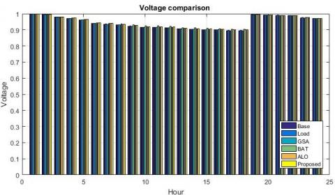
Figure 5. Comparison analysis of voltages using various methods for 24 hours on IEEE-33 bus system
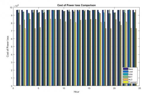
The Comparison Analysis of load line power loss using various methods connected in different DGs from different time period is illustrated in Figures 5 to 12. From the simulation outcomes it may be observed that low active power losses and improved voltage at each bus was achieved by the connection of DGs at the optimal place obtained by VSI using various approaches. Overall loss reduction is accomplished with the integration of DGs utilizing the projected technique which is much superior than the power loss of different techniques. Hence, this can be concluded that improved ALO technology is much effective than other technologies in reduction of power loss of IEEE-33 and IEEE-69 standard radial distribution system.
Figure 6. Comparison analysis of loss of power using various methods for 24 hours on IEEE-33 bus system
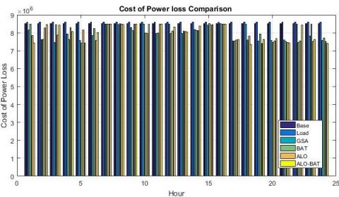
Figure 7. Comparison analysis of cost of loss of power using various methods for 24 hours on IEEE-33 bus system
Figure 8. Comparative analysis of cost of DG various methods for 24 hours on IEEE-33 bus system
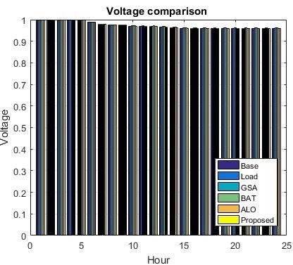
Figure 9. Comparison analysis of voltages using various methods for 24 hours on IEEE-69 bus system
Figure 10. Comparative analysis of cost of DG using various methods for 24 hours on IEEE-69 bus system
Figure 11. Comparison analysis of loss of power using various methods for 24 hours on IEEE-69 bus system
Figure 12. Comparison analysis of cost of loss of power using various Methods for 24 hours on IEEE-69 bus system
Here, the DG in a RDS is connected in an optimal location and capacity, which is estimated based on the efficient technique. This technique is improved ALO algorithm, which is the performance is improved by using the Bat algorithm. The projected approach is capable of provide much competitive outcomes in terms of updated exploration, local optima avoidance, exploitation and convergence. The ALO approach is also determine best optimal approaches for the majority of classical engineering issues employed, proving that this approach has advantages in solving constrained issues with diverse search spaces. Then the performance of the ALO is improved with the help of BA. The reactive power capability of PV network, wind turbines are considered in the voltage control. To evaluate the performance of the proposed system, an ALO technique based on the BA is also performed to obtain the best reactive power output of the DGs. The proposed control network is also applied to the IEEE-33 and IEEE-69 distribution scheme to show the robustness of the projected technique. The outcomes proves that the projected approach is much effective, and has a better fitness function, and has comparable time of convergence with GSA and capability to handle complex optimization issues. In addition, projected approach is much efficient in terms of loss minimization, voltage enhancement and load ability enhancement of distribution scheme. The efficiency of the projected technique is determined and compared with the existing techniques.
|
Nn |
Numbaer of system buses |
|
Vni |
specifies the ith bus voltage |
|
Vrated |
rated bus voltage |
|
Pgni |
generator output real power at ni bus |
|
Pdni |
demand of real power at ni bus |
|
Vmi |
voltage of mi bus |
|
Vni |
voltage of ni bus |
|
Ymni |
admittance magnitude among mi bus and ni bus |
|
Nbus |
number of buses |
|
ni |
receiving bus number |
|
mi |
bus number that sending power |
|
i |
branch number that fed ni bus |
|
PGi |
real power generated at bus i |
|
QGi |
reactive power generated at bus i |
|
PDi |
real load demand at bus i |
|
QDi |
reactive load demand at bus i |
|
Pi |
real injected power at bus i |
|
Qi |
reactive injected power at bus i |
|
Yij |
magnitude of admittance |
|
Vmax |
peak voltage at bus |
|
Vmin |
lowest voltage at bus |
|
Vi |
current node voltage |
|
Vi+1 |
voltage at next bus |
|
Pi+1 |
next node active power |
|
Qi+1 |
next node reactive power |
|
Ri |
line resistance among i and i+1 node |
|
Xi |
line reactance line among i and i+1 node |
|
Greek symbols |
|
|
δmi |
voltage phase angle at mi bus |
|
δni |
voltage phase angle at ni bus |
|
θni |
angle of admittance |
|
θij |
branch voltage angle |
|
Subscripts |
|
|
DG |
Distributed generation |
|
WT |
Wind turbine |
|
PV |
Photo-voltaic |
|
BW/FW |
Backward and farward sweep |
|
GSA |
Gravitational search algorithm |
|
BA |
Bat algorithm |
|
ALO |
Ant-lion optimization |
|
AI |
Artificial intelligance |
|
OPF |
Optimal power flow |
|
kW |
Kilo watt |
|
p.u |
Per unit |
|
MOPSO |
Multi-objective particle swarm optimization |
|
PSO |
Particle swarm optimization |
|
GA |
Genetic algorithm |
|
VSI |
Voltage stabilty index |
[1] Biswas, S., Goswami, S.K., Chatterjee, A. (2012). Optimum distributed generation placement with voltage sag effect minimization. An International Journal of Energy Conversion and Management, 53(1): 163-174. http://doi.org/10.1016/j.enconman.2011.08.020
[2] Muttaqi, K., Le, A.D., Negnevitsky, M., Ledwich, G. (2014). An algebraic approach for determination of DG parameters to support voltage profiles in radial distribution networks. IEEE Transactions on Smart Grid, 5(3): 1351-1360. http://doi.org/10.1109/TSG.2014.2303194
[3] Moradi, M.H., Abedini, M. (2012). A combination of genetic algorithm and particle swarm optimization for optimal DG location and sizing in distribution systems. An International Journal of Electrical Power and Energy Systems, 34: 66-74. http://doi.org/10.1109/IPECON.2010.5697086
[4] Sultana, U., Khairuddin, A.B., Aman, M.M., Mokhtar, A.S., Zareen, N. (2016). A review of optimum DG placement based on minimization of power losses and voltage stability enhancement of distribution system. An International Journal of Renewable and Sustainable Energy Reviews, 63: 363-378. http://doi.org/10.1016/j.rser.2016.05.056
[5] Reddy, S.C., Prasad, P.V.N., Laxmi, A.J. (2012). Reliability improvement of distribution system by optimal placement of DGs using PSO and neural network. In proceedings of International Conference on Computing, Electronics and Electrical Technologies [ICCEET]. http://doi.org/10.1109/ICCEET.2012.6203836
[6] Jabr, R.A., Pal, B.C. (2009). Ordinal optimisation approach for locating and sizing of distributed generation. IET Generation, Transmission, Distribution, 3(8): 713-723. http://doi.org/10.1049/iet-gtd.2009.0019
[7] Priya, R., Prakash, S. (2014). Optimal location and sizing of generator in distributed generation system. An International Journal of Innovative Research in Electrical, Electronics, Instrumentation and Control Engineering 2(3): 1-5.
[8] Nayanatara, C., Baskaran, J., Kothari, D.P. (2016). Hybrid optimization implemented for distributed generation parameters in a power system network. An International Journal of Electrical Power and Energy Systems, 78: 690-699. http://doi.org/10.1016/j.ijepes.2015.11.117
[9] García, J.A.M., Mena, A.J.G. (2013). Optimal distributed generation location and size using a modified teaching–learning based optimization algorithm. An International Journal of Electrical Power and Energy Systems, 50: 65-75. http://doi.org/10.1016/j.ijepes.2013.02.023
[10] Abu-Mouti, F.S., El-Hawary, M.E. (2011). Heuristic curve-fitted technique for distributed generation optimisation in radial distribution feeder systems. IET Generation, Transmission, Distribution, 5(2): 172-180. http://doi.org/10.1049/iet-gtd.2009.0739
[11] Bharathi Dasan, S.G., Selvi Ramalakshmi, S., Kumudini Devi, R.P. (2009). Optimal siting and sizing of hybrid distributed generation using EP. In proceedings of 3rd International Conference on Power Systems, Kharagpur, India. http://doi.org/10.1109/ICPWS.2009.5442761
[12] Mahipal, B., Naik, G.B., Kumar, C.N. (2016). A novel method for determining optimal location and capacity of dg and capacitor in radial network using weight-improved particle swarm optimisation algorithm (WIPSO). An International Journal of Advanced Research in Electrical, Electronics and Instrumentation Engineering, 5(5): 3478-3485. http://doi.org/10.15662/IJAREEIE.2016.0505004
[13] Linh, N.T., Dong, D.X. (2013). Optimal location and size of distributed generation in distribution system by artificial bees colony algorithm. An International Journal of Information and Electronics Engineering, 3(1): 63-67. http://doi.org/10.7763/IJIEE.2013.V3.267
[14] El-Zonkoly, A.M. (2011). Optimal placement of multi-distributed generation units including different load models using particle swarm optimization. IET Generation, Transmission, Distribution, 5(7): 760-771. https://doi.org/10.1016/j.swevo.2011.02.003
[15] Samala, R.K., Kotapuri, M.R. (2018). Distributed generation in distribution system for power quality enhancement. International Journal of Engineering & Technology, 7: 167-171. http://doi.org/10.14419/ijet.v7i4.24.21881
[16] Samala, R.K., Kotapuri, M.R. (2020). Optimal allocation of distributed generations using hybrid technique with fuzzy logic controller radial distribution system. SN Applied Sciences, 2: 191. https://doi.org/10.1007/s42452-020-1957-3.
[17] Narayanan, K., Siddiqui, S.A., Fozdar, M. (2015). Identification and reduction of impact of islanding using hybrid method with distributed generation. In proceedings of IEEE Power & Energy Society General Meeting, pp. 1-5. http://doi.org/10.1109/PESGM.2015.7286467
[18] Gomez-Gonzalez, M., Lopez, A., Jurado, F. (2012). Optimization of distributed generation systems using a new discrete PSO and OPF. An International Journal of Electric Power Systems Research, 84: 174-180. http://doi.org/10.1016/j.epsr.2011.11.016
[19] Kotapuri, M.R., Samala, R.K. (2020). Distributed generation allocation in distribution system using particle swarm optimization based ant-lion optimization. International Journal of Control and Automation, 13(1): 414-426.
[20] Prakash, P., Khatod, D.K. (2016). Optimal sizing and siting techniques for distributed generation in distribution systems: A review. An International Journal of Renewable and Sustainable Energy Reviews, 57: 111-130. http://doi.org/10.1016/j.rser.2015.12.099
[21] Rezaei, F., Esmaeili, S. (2017). Decentralized reactive power control of distributed PV and wind power generation units using an optimized fuzzy-based method. An International Journal of Electrical Power and Energy Systems, 87: 27-42. https://doi.org/10.1016/j.ijepes.2016.10.015
[22] Jamian, J.J., Mustafa, M.W., Mokhlis, H., Baharudin, M.A., Abdilahi, A.M. (2014). Gravitational search algorithm for optimal distributed generation operation in autonomous network. Arabian Journal for Science and Engineering, 39: 7183-7188. http://doi.org/10.1007/s13369-014-1279-0
[23] Rama Prabha, D., Jayabarathi, T., Umamageswari, R., Saranya, S. (2015). Optimal location and sizing of distributed generation unit using intelligent water drop algorithm. An International Journal of Sustainable Energy Technologies and Assessments, 11: 106-113. http://doi.org/10.1016/j.seta.2015.07.003