Vu Trieu Minh | Mart Tamre | Victor Musalimov | Pavel Kovalenko | Irina Rubinshtein | Ivan Ovchinnikov | David Krcmarik | Reza Moezzi* | Jaroslav Hlava
© 2020 IIETA. This article is published by IIETA and is licensed under the CC BY 4.0 license (http://creativecommons.org/licenses/by/4.0/).
OPEN ACCESS
Human muscles and the central nervous system (CNS) play the key role to control the human movements and activities. The human CNS determines each human motion following three steps: estimation of the movement trajectory; calculation of required energy for muscles; then perform the motion. In these three step tasks, the human CNS determines the first two steps and the human muscles conduct the third one. This paper efforts the use of model predictive control (MPC) algorithm to simulate the human CNS calculation in the case of gait motion. We first build up the human gait motion mathematical model with 5-link mechanism. This allows us to apply MPC to calculate the optimal torques at each joint and optimal trajectory for muscles. Outcomes of simulations simultaneously are compared with the real human movements captured by the Vicon motion capture technology which is the novelty of this study. Results show that tracking errors are not excessed 7%.
human gait plant, human gait model, central nervous system, model predictive control, 5-link mechanism, Vicon motion capture
Human gait motions are performed consequently by the central nervous system (CNS), muscles, and limbs. In recent years, there are many researches on modeling human gait motions for mimicking the real human trajectories and/or the walking patterns, even though, each person has its inimitable gait motion and/or the gait of each individual person is unique. Most of design and development of human gait are based on the intuition, followed by experimental verifications [1]. These approaches are usually costly, unsustainable and ineffective.
In the fields such as Medicine, Psychology and especially Biomechanics, investigation on human motion gaits can resolve many problems [2, 3]. for example, a doctor can check his assumptions about a disease of the limbs without costly testing experimentations on patient. The real human gait modeling can also simplify the process of checking orthotic devices and artificial limbs or using humanoid robot. These parts are normally tested empirically and expensively.
The cyclic motion of human gait is involving of two phases: the stance phase and the swing phase. Discussion on the phases and their occurrence is out of scope of this study (which is mostly related to medical field), but the basic understanding can improve the intuitive considerate of the problem [4]. This study aims to develop a simple but flexible solution to control the human gait used by MPCs. Thanks to computer based numerical solutions which has increasingly provide optimization-based control algorithm. MPC has lots of advantages in different fields. Simulations of this method can be regulated with different MPC parameters and objective functions. Real data are obtained by the motion capture Vicon cameras which this device has not been simultaneously used to capture and compare with the mathematical model. We first start reviewing some recent developments on modeling human as well as issues related to new productions of orthoses and prostheses for human climbs.
A new modeling based on a kinematics of human body from data achieved by a camera of optoelectronic system for measuring three dimensions is developed by Vergallo et al. [5], where sophisticated software is used to convert the images of human walking based on appropriate protocols to describe the human motions in each joint. A human gait model used the biomechanical principles of Lagrange method for reproducing the properties of human walking is presented in the paper [6], where anthropometric data are used to simulate the human walking dynamics. Comparisons of the model simulations and the real camera measurements show that the model can reproduce accurate characteristics of the gait motions. Several approaches involving the use of three-dimensional cameras and image processing have been introduced. However, a less expensive method for using the infrared depth camera for modeling the human gait is presented in spaces with low or no light conditions with passive sensors [7]. The cost for this method is low but the advantages and precision of this method are still unclear. A PhD dissertation on dynamic modeling of human gait using a model predictive control approach is presented by Sun [8], where a plant model for the human gait dynamics is built and a control feedback with PID and MPC is designed for simulating the human gaits. This control-based simulation method provides unlimited flexible gaits. However, the disadvantage of this method is unable to ensure the stability and robustness of the model.
Majority of numerical researches are used the Lagrange equations to describe the motions of limbs and modeling the gaits as the position of a 5-link, 7-link, or 9-link mechanism. However, there are limitations from these methods that they are unable to include constraints of dynamic equations such as the mass density and centers. For example, some good results, which are almost matching the experimental data, are achieved, but paths of some point motions are totally incorrect, and the computations are very difficult [9]. Therefore, a predictive modeling of human walking over a complete gait is presented [10]. The shortcomings of mentioned study are the lack of constrained conditions and fails to develop an objective function, that is able to minimized the energy cost.
A completed control function for arm swing and human walking is developed by Pontzer et al. [11] with a proposal that the arm acts as a passive mass damper and powered by the movement of the human lower body. While Mohammed et al. [12] develops the recognition of gaits using wearable sensors. This paper monitors the human walking through the analysis of the human center of force and predicts any abnormal walking pattern. Identification of different gaits is detected from characteristics of gait phases.
In this research, a mathematic model describing the path of movement of the anthropomorphic mechanism is developed for analyzing solutions, which is close (but not sufficient) to the real. Then, MPC algorithms are designed to calculate the optimal energy for muscles. It is assumed that the human walking is a 5-link mechanism model and the CNS is trying to predict and calculate the lower extremities (feet, shins, hips, and body) to perform the movements. MPC is used to calculate the optimal controller torques for muscles. MPC algorithms for nonlinear models and different MPC computational schemes are mainly referred in the paper [13] where the NMPC performances using a terminal region scheme, NMPC with quasi-infinite scheme, and NMPC without soften state constraints scheme are simulated and compared. In this paper, the NMPC algorithms with soften state constraints are used for calculated the optimal torques in joints. For simulating the human dynamics in MATLAB, Simulink, some mechanical mechanisms in the paper [14] are used for building the human plant. Latest human gait engineering studies are referred to in the papers [15-18]. Other control strategies beside NMPC [19], also can be considered, such as Adaptive Control Strategy, fuzzy based control [20], tracking control based on NMPC or neural network, but based on the simplicity of the MPC, it’s the most convenient method for the human gait motion investigation.
The structure of this paper is as follows: Section 2 briefs the mathematical modeling; Section 3 designs MPC controller model; Section 4 designs the plant model; in Section 5 results of simulation are provided; And finally, conclusions and recommendations are withdrawn in Section 6.
The mathematical model of 5-link mechanism is shown in Figure 1. This model is used for MPC controller to calculate the optimal controller torques for each joint. Five weighty links are OC, OB, OD, DE, and BE. Link OC is the body. ODE and OBA are feet. Each leg consists of the thigh and lower leg, so that the link OB and OD are hips and unit’s BA and DE are shins. Two legs are considered of the same weight and length.
Figure 1. Model of 5-link mechanism
Joint O connecting the body OC with hips OB and OD will be referred as hip joint, joints B and D, connecting the thigh OB and OD with shins BA and DE, will be referred as knee joints. All joints are assumed to be ideal, i.e. friction in their neglect. This mechanism has seven degrees of freedom. In describing the situation as six generalized coordinates, we choose the following works: coordinates x, y of hip О and five angles ψ, α_1, α_2, β_1, β_2, between the links and the vertical. These angles and directions of their reference are shown in Figure 1: ψ – the angle between the body and the vertical, α_1 and β_1 – the angles between the hips and the vertical, β_1, and β_2, – the angles formed by the vertical tibia. The angle is positive when the relevant unit deviates from the vertical direction in the opposite clockwise direction.
For this simplified model of 5-link, human feet have a small part of all mass, and we may assume that the feet do not have a strong influence on the movement of other parts of human. The following equations are used directly in the system for calculation.
Lagrange equation:
$\frac{d}{d t} \cdot \frac{\partial L}{\partial \dot{q}_{i}}-\frac{\partial L}{\partial q_{i}}=Q_{s}$ (1)
where, Qs - generalizes non conservative force, and
$L=T-V$ (2)
where, L - Lagrangian; T – kinetic energy; V - potential energy;
Kinetic energy:
$T=\frac{1}{2}\left(m v^{2}+2 m(v \omega) p+\Theta \omega^{2}\right)$ (3)
where, m - mass of link; v - absolute velocity; v - pole velocity; w - angular velocity; p - radius vector of the center of mass; $\Theta$ - Inertia moment relative to pole.
$v=\left(\begin{array}{c}\dot{x} \\ \dot{y} \\ 0\end{array}\right)$ (4)
$\omega={\psi}\left(\begin{array}{c}\sin (\psi) \\ \cos (\psi) \\ 0\end{array}\right)$ (5)
inetic energy of link OC point O is a pole, so:
$T_{O C}=\frac{1}{2}\left(\begin{array}{c}m_{k}\left(\dot{x}^{2}+\dot{y}^{2}\right)- \\ 2 K_{r} \dot{\psi}(\dot{x} \cos (\psi)+\dot{y} \sin (\psi))+J \dot{\psi}^{2}\end{array}\right)$ (6)
where, $K_{r}=m_{k} r$; $\mathrm{m}_{\mathrm{k}}$ - Mass OC; r - distance from O to OC mass center; J - inertia moment OC relative point O.
In finding the kinetic energy for the body OC and hips OB and OD, a pole will take at the point O. Similarly, for parts of BA and DE, the pole point B and D are chosen. For kinetic energy of link OB, point O is chosen as a pole, so:
$T_{O B}=\frac{1}{2}\left(m_{a}\left(\dot{x}^{2}+\dot{y}^{2}\right)\right.$$+2 m_{a} a \dot{\alpha_{1}}\left(\dot{x} \cos \left(\alpha_{1}\right)\right.$$\left.\left.+\dot{y} \sin \left(\alpha_{1}\right)\right)+J_{a}^{0} \dot{\alpha_{1}}^{2}\right)$ (7)
where, $m_{a}$ - mass OB; a - distance from O to OB mass centre; $J_{a}^{0}$ - inertia moment OB relative point O.
Kinetic energy of link BA point B:
$T_{B A}=\frac{1}{2}\left(m_{b}\left(\dot{x}^{2}+\dot{y}^{2}\right.\right.$$+2 \dot{\alpha_{1}} L_{a}\left(\dot{x} \cos \left(\alpha_{1}\right)+\dot{y} \sin \left(\alpha_{1}\right)\right)$$\left.+L_{a}^{2} \dot{\alpha_{1}}^{2}\right)$$+2 K_{b} \dot{\beta}_{1}\left(\dot{x} \cos \left(\beta_{1}\right)+\dot{y} \sin \left(\beta_{1}\right)\right)$$\left.+J_{b} \dot{\beta}_{1}^{2}\right)$ (8)
where, $K_{b}=m_{b} b$; $\mathrm{m}_{\mathrm{b}}$ - mass BA; b - distance from B to BA mass center; $L_{a}$ - length of OB; Jb - inertia moment BA relative point B.
TOD and TDE can be taken from TOB and TBA by changing indexes from 1 to 2:
$\begin{aligned} T=T_{O C}+T_{O B}+& T_{B A}+T_{O D}+T_{D E} \\ &=\frac{1}{2} M\left(\dot{x}^{2}+\dot{y}^{2}\right)+\frac{1}{2} J {\psi}^{2} \\ &-K_{r} {\psi}(\dot{x} \cos (\psi)+\dot{y} \sin (\psi)) \\ &+\sum_{i=1}^{2}\left[\frac{1}{2} J_{a} \dot{\alpha}_{l}^{2}+\frac{1}{2} J_{b} \dot{\beta}_{l}^{2}\right.\\ &+K_{a} \dot{\alpha}_{\iota}\left(\dot{x} \cos \left(\alpha_{i}\right)+\dot{y} \sin \left(\alpha_{i}\right)\right) \\ &+K_{b} \dot{\beta}_{l}\left(\dot{x} \cos \left(\beta_{i}\right)+\dot{y} \sin \left(\beta_{i}\right)\right) \\ &\left.+J_{a b} \dot{\alpha}_{l} \dot{\beta}_{l} \cos \left(\alpha_{i}-\beta_{i}\right)\right] \end{aligned}$ (9)
where,
$M=m_{k}+2 m_{a}+2 m_{b}-$total mass (10)
$K_{a}=m_{a} a+m_{b} L_{a}$ (11)
$J_{a}=J_{a}^{0}+m_{b} L_{a}^{2}$ (12)
$J_{a b}=K_{b} L_{a}=m_{b} b L_{a}$ (13)
Potential energy:
$V=g\left[m_{k}(y+r \cos (\psi))\right.$$+\sum_{i=1}^{2}\left(m_{a}\left(y-a \cos \left(\alpha_{i}\right)\right)\right.$$\left.\left.+m_{b}\left(y-L_{a} \cos \left(\alpha_{i}\right)-b \cos \left(\beta_{i}\right)\right)\right)\right]$$=g\left[M y+K_{r} \cos (\psi)\right.$$\left.-\sum_{i=1}^{2}\left(K_{a} \cos \left(\alpha_{i}\right)+K_{b} \cos \left(\beta_{i}\right)\right)\right]$ (14)
In this paper, MPC algorithms are used to find the optimal trajectory based on the minimization of an objective function and subject to constraints. Therefore, from Eq. (1), we find T and V, next we need to find QS by following some elementary expressions:
$\delta W=\left(R_{1 x}+R_{2 x}\right) \delta x+\left(R_{1 y}+R_{2 y}\right) \delta y$$-\left(q_{1}+q_{2}\right) \delta \psi$$\quad+\sum_{i=1}^{2}\left[\left(q_{i}-u_{i}\right) \delta \alpha_{i}\right.$$\quad+\left(u_{i}-P_{i}\right) \delta \beta_{i}$$\quad+R_{1 x} \delta\left(L_{a} \sin \left(\alpha_{i}\right)+L_{b} \sin \left(\beta_{i}\right)\right)$$\quad-R_{1 y} \delta\left(L_{a} \cos \left(\alpha_{i}\right)\right.$$\left.\left.\quad+L_{b} \cos \left(\beta_{i}\right)\right)\right]$
$=\sum_{i=1}^{2}\left[R_{i x} \delta x+R_{i y} \delta y-q_{i} \delta \psi\right.$$+\left(q_{i}-u_{i}\right.$$+R_{1 x} L_{a} \cos \left(\alpha_{i}\right)$$\left.+R_{1 y} L_{a} \sin \left(\alpha_{i}\right)\right) \delta \alpha_{i}$$+\left(u_{i}-P_{i}\right.$$+R_{1 x} L_{b} \cos \left(\beta_{i}\right)$$\left.\left.+R_{1 y} L_{b} \sin \left(\beta_{i}\right)\right) \delta \beta_{i}\right]$ (15)
where,
$Q_{x}=R_{1 x}+R_{2 x}$ (16)
$Q_{y}=R_{1 y}+R_{2 y}$ (17)
$Q_{\psi}=-q_{1}-q_{2}$ (18)
$Q_{\alpha_{1}}=q_{1}-u_{1}+R_{1 x} L_{a} \cos \left(\alpha_{1}\right)+R_{1 y} L_{a} \sin \left(\alpha_{1}\right)$ (19)
$Q_{\alpha_{2}}=q_{2}-u_{2}+R_{1 x} L_{a} \cos \left(\alpha_{2}\right)+R_{1 y} L_{a} \sin \left(\alpha_{2}\right)$ (20)
$Q_{\beta_{1}}=u_{1}-P_{1}+R_{1 x} L_{b} \cos \left(\beta_{1}\right)+R_{1 y} L_{b} \sin \left(\beta_{1}\right)$ (21)
$Q_{\beta_{2}}=u_{2}-P_{2}+R_{1 x} L_{b} \cos \left(\beta_{2}\right)+R_{1 y} L_{b} \sin \left(\beta_{2}\right)$ (22)
The derivatives of these variables can be described as follows:
Derivative $\frac{\partial \mathrm{L}}{\partial \mathrm{z}}$ :
$\frac{\partial L}{\partial x}=\frac{\partial(T-V)}{\partial x}=0$ (23)
$\frac{\partial L}{\partial y}=\frac{\partial(T-V)}{\partial y}=-g M$ (24)
$\frac{\partial L}{\partial \psi}=\frac{\partial(T-V)}{\partial \psi}=K_{r}(\dot{x} {\psi} \sin (\psi)-\dot{y} {\psi} \cos (\psi)$$-g \sin (\psi))$ (25)
$\frac{\partial L}{\partial \alpha_{i}}=\frac{\partial(T-V)}{\partial \alpha_{i}}=K_{a}\left(\dot{\alpha}_{l} \dot{x} \sin \left(\alpha_{i}\right)\right.$$\left.-\dot{\alpha}_{l} \dot{y} \cos \left(\alpha_{i}\right)+g \sin \left(\alpha_{i}\right)\right)$$-J_{a b} \dot{\alpha}_{l} \dot{\beta}_{l} \sin \left(\alpha_{i}-\beta_{i}\right)$ (26)
$\frac{\partial L}{\partial \beta_{i}}=\frac{\partial(T-V)}{\partial \beta_{i}}=K_{b}\left(\dot{\beta}_{l} \dot{x} \sin \left(\beta_{i}\right)\right.$$\left.-\dot{\beta}_{l} \dot{y} \cos \left(\beta_{i}\right)+g \sin \left(\beta_{i}\right)\right)$$-J_{a b} \dot{\alpha}_{l} \dot{\beta}_{l} \sin \left(\alpha_{i}-\beta_{i}\right)$ (27)
Derivative $\frac{\partial \mathrm{L}}{\partial \dot{\mathrm{z}}}$:
$\frac{\partial L}{\partial \dot{x}}=M \dot{x}-K_{r} \dot{\psi} \cos (\psi)+K_{a} \dot{\alpha}_{i} \cos \left(\alpha_{i}\right)+K_{b} \dot{\beta}_{i} \cos \left(\beta_{i}\right)$ (28)
$\frac{\partial L}{\partial \dot{y}}=M \dot{y}-K_{r} \dot{\psi} \sin (\psi)+K_{a} \dot{\alpha}_{i} \sin \left(\alpha_{i}\right)+K_{b} \dot{\beta}_{i} \sin \left(\beta_{i}\right)$ (29)
$\frac{\partial L}{\partial \dot{\psi}}=J \dot{\psi}-K_{r}(\dot{x} \cos (\psi)+\dot{y} \sin (\psi))$ (30)
$\frac{\partial L}{\partial \dot{\alpha}_{i}}=J_{a} \dot{\alpha}_{i}+K_{a}\left(\dot{x} \cos \left(\alpha_{i}\right)+\dot{y} \sin \left(\alpha_{i}\right)\right)+J_{a b} \dot{\beta}_{i} \cos \left(\alpha_{i}-\beta_{i}\right)$ (31)
$\frac{\partial L}{\partial \dot{\beta}_{i}}=J_{b} \dot{\beta}_{i}+K_{b}\left(\dot{x} \cos \left(\beta_{i}\right)+\dot{y} \sin \left(\beta_{i}\right)\right)+J_{a b} \dot{\alpha}_{i} \cos \left(\alpha_{i}-\beta_{i}\right)$ (32)
Derivatives: $\frac{d}{d t} \frac{\partial L}{\partial \dot{z}}$ :
$\begin{aligned} \frac{d}{d t} \frac{\partial L}{\partial \dot{x}}=M \ddot{x}-K_{r} \ddot{\psi} & \cos (\psi)+K_{r} \dot{\psi}^{2} \sin (\psi) \\ &+K_{a} \ddot{\alpha}_{l} \cos \left(\alpha_{i}\right)-K_{a} \dot{\alpha}_{l}^{2} \sin \left(\alpha_{i}\right) \\ &+K_{b} \ddot{\beta}_{l} \cos \left(\beta_{i}\right)-K_{b} \dot{\beta}_{l}^{2} \sin \left(\beta_{i}\right) \end{aligned}$ (33)
$\begin{aligned} \frac{d}{d t} \frac{\partial L}{\partial \dot{y}}=M \ddot{y}-K_{r} \ddot{\psi} & \sin (\psi)-K_{r} \dot{\psi}^{2} \cos (\psi) \\ &+K_{a} \ddot{\alpha}_{l} \sin \left(\alpha_{i}\right)+K_{a} \dot{\alpha}_{l}^{2} \cos \left(\alpha_{i}\right) \\ &+K_{b} \ddot{\beta}_{l} \sin \left(\beta_{i}\right)+K_{b} \dot{\beta}_{l}^{2} \cos \left(\beta_{i}\right) \end{aligned}$ (34)
$\begin{aligned} \frac{d}{d t} \frac{\partial L}{\partial \dot{\psi}}=J \ddot{\psi}-K_{r}(\ddot{x} \cos (\psi)\\ &+\ddot{y} \sin (\psi)-\dot{x} \dot{\psi} \sin (\psi) \\ &+\dot{y} \dot{\psi} \cos (\psi)) \end{aligned}$ (35)
$\frac{d}{d t} \frac{\partial L}{\partial \dot{\alpha}_{l}}=J_{a} \ddot{\alpha}_{l}+K_{a}\left(\ddot{x} \cos \left(\alpha_{i}\right)\right.$$+\ddot{y} \sin \left(\alpha_{i}\right)+\dot{x} \dot{\alpha}_{l} \sin \left(\alpha_{i}\right)$$\left.-\dot{y} \dot{\alpha}_{l} \cos \left(\alpha_{i}\right)\right)$$+J_{a b} \ddot{\beta}_{l} \cos \left(\alpha_{i}-\beta_{i}\right)-J_{a b} \dot{\beta}_{l}\left(\alpha_{i}\right.$$\left.-\beta_{i}\right) \sin \left(\alpha_{i}-\beta_{i}\right)$ (36)
$\frac{d}{d t} \frac{\partial L}{\partial \dot{\beta}_{l}}=J_{b} \ddot{\beta}_{l}+K_{b}\left(\ddot{x} \cos \left(\beta_{i}\right)\right.$$+\ddot{y} \sin \left(\beta_{i}\right)+\dot{x} \beta_{i} \sin \left(\beta_{i}\right)$$\left.-\dot{y} \beta_{i} \cos \left(\beta_{i}\right)\right)+J_{a b} \ddot{\alpha}_{l} \cos \left(\alpha_{i}-\beta_{i}\right)$$-J_{a b} \alpha_{l}\left(\alpha_{l}-\beta_{l}\right) \sin \left(\alpha_{i}-\beta_{i}\right)$ (37)
And finally, full Lagrange equations for this 5–link mechanism:
$\begin{aligned} M \ddot{x}-K_{r} \ddot{\psi} \cos (\psi) &+K_{r} \dot{\psi}^{2} \sin (\psi) \\ &+K_{a} \ddot{\alpha}_{l} \cos \left(\alpha_{i}\right)-K_{a} \dot{\alpha}_{l}^{2} \sin \left(\alpha_{i}\right) \\ &+K_{b} \ddot{\beta}_{l} \cos \left(\beta_{i}\right)-K_{b} \dot{\beta}_{l}^{2} \sin \left(\beta_{i}\right) \\ &=R_{1 x}+R_{2 x}, \quad(i=1,2) \end{aligned}$ (38)
$\begin{aligned} M \ddot{y}-K_{r} \ddot{\psi} \sin (\psi) &-K_{r} \dot{\psi}^{2} \cos (\psi)+K_{a} \ddot{\alpha}_{l} \sin \left(\alpha_{i}\right) \\ &+K_{a} \dot{\alpha}_{l}^{2} \cos \left(\alpha_{i}\right) \\ &+K_{b} \ddot{\beta}_{l} \sin \left(\beta_{i}\right)+K_{b} \dot{\beta}_{l}^{2} \cos \left(\beta_{i}\right) \\ &=R_{1 y}+R_{2 y}-M g, \quad(i=1,2) \end{aligned}$ (39)
$-K_{r} \ddot{x} \cos (\psi)-K_{r} \ddot{y} \sin (\psi)+J \ddot{\psi}-K_{r} g \sin (\psi)$$=-q_{1}-q_{2}, \quad(i=1,2)$ (40)
$\begin{aligned} K_{a} \ddot{x} \cos \left(\alpha_{i}\right)+K_\ddot{a} y & \sin \left(\alpha_{i}\right)+J_{a} \ddot{\alpha}_{l} \\ &+J_{a b} \ddot{\beta}_{l} \cos \left(\alpha_{i}-\beta_{i}\right) \\ &+J_{a b} \dot{\beta}_{l} \sin \left(\alpha_{i}-\beta_{i}\right) \\ &+K_{a} g \sin \left(\alpha_{i}\right) \\ &=q_{i}-u_{i} \\ &+R_{1 x} L_{a} \cos \left(\alpha_{i}\right) \\ &+R_{1 y} L_{a} \sin \left(\alpha_{i}\right),(i=1,2) ; \end{aligned}$ (41)
$K_{b} \ddot{x} \cos \left(\beta_{i}\right)+K_{b} \ddot{y} \sin \left(\beta_{i}\right)+J_{b} \ddot{\beta}_{l}+J_{a b} \ddot{\alpha}_{l} \cos \left(\alpha_{i}-\beta_{i}\right)$$-J_{a b} \dot{\alpha}_{l}^{2} \sin \left(\alpha_{i}-\beta_{i}\right)+K_{b} g \sin \left(\beta_{i}\right)$
$=u_{i}-P_{i}$$+R_{1 x} L_{b} \cos \left(\beta_{i}\right)$$+R_{1 y} L_{b} \sin \left(\beta_{i}\right), \quad(i=1,2)$ (42)
These equations describe the dynamics of 5-link model, but the model has limited movement as point A or E being fixed on the surface:
If point A fixed, we have kinematic equations for x and y:
$x=x_{A}-L_{a} \sin \left(\alpha_{1}\right)-L_{b} \sin \left(\beta_{1}\right)$ (43)
$y=y_{A}+L_{a} \cos \left(\alpha_{1}\right)+L_{b} \cos \left(\beta_{1}\right)$ (44)
$\dot{x}=-L_{a} \dot{\alpha}_{1} \cos \left(\alpha_{1}\right)-L_{b} \dot{\beta}_{1} \cos \left(\beta_{1}\right)$ (45)
$\dot{y}=-L_{a} \dot{\alpha_{1}} \sin \left(\alpha_{1}\right)-L_{b} \dot{\beta}_{1} \sin \left(\beta_{1}\right)$ (46)
New equations for T, V and $\delta W$ in (9, 14) for (43 to 46):
$T=\frac{1}{2} J \dot{\psi}^{2}+\frac{1}{2} M\left(J_{a}-2 L_{a} K_{a}+L_{a}^{2} M\right) \dot{\alpha_{1}}^{2}+\frac{1}{2} J_{a} \dot{\alpha_{2}}^{2}$$+\frac{1}{2} M\left(J_{b}-2 L_{b} K_{b}+L_{b}^{2} M\right) \dot{\beta_{1}}^{2}$$+\frac{1}{2} J_{a} \dot{\beta}_{2}^{2}+L_{a} K_{r} \cos \left(\psi-\alpha_{1}\right) \dot{\psi} \dot{\alpha}_{1}$
$+L_{b} K_{r} \cos \left(\psi-\beta_{1}\right) \dot{\psi} \dot{\beta}_{1}$$-L_{a} K_{a} \cos \left(\alpha_{1}-\alpha_{2}\right) \dot{\alpha}_{1} \dot\alpha_{2}$$+\left(J_{a b}-L_{a} K_{b}-L_{b} K_{a}\right.$$\left.+L_{a} L_{b} M\right) \cos \left(\alpha_{1}-\beta_{1}\right) \dot{\alpha}_{1} \dot{\beta}_{1}$ (47)
$-L_{a} K_{b} \cos \left(\alpha_{1}-\beta_{2}\right) \dot{\alpha}_{1} \dot{\beta}_{2}$$-L_{b} K_{a} \cos \left(\alpha_{2}-\beta_{1}\right) \dot{\alpha}_{2} \dot{\beta}_{1}$$+L_{b} K_{b} \cos \left(\beta_{1}-\beta_{2}\right) \dot{\beta}_{1} \dot{\beta}_{2}$
$V=g\left[M y_{A}+K_{r} \cos (\psi)+\left(L_{a} M-K_{a}\right) \cos \left(\alpha_{1}\right)\right.$$-K_{a} \cos \left(\alpha_{2}\right)$$+\left(L_{b} M-K_{b}\right) \cos \left(\beta_{1}\right)$$\left.-K_{b} \cos \left(\beta_{2}\right)\right]$ (48)
$\begin{aligned} \delta W=-\left(q_{1}+q_{2}\right) & \delta \psi \\+&\left(q_{1}-u_{1}-R_{2 x} L_{a} \cos \left(\alpha_{1}\right)\right.\\-&\left.R_{2 y} L_{a} \sin \left(\alpha_{1}\right)\right) \delta \alpha_{1} \\ &+\left(q_{2}-u_{2}-R_{2 x} L_{a} \cos \left(\alpha_{2}\right)\right.\\ &\left.-R_{2 y} L_{a} \sin \left(\alpha_{2}\right)\right) \delta \alpha_{2} \\ &+\left(u_{1}-P_{1}-R_{2 x} L_{b} \cos \left(\beta_{1}\right)\right.\\ &\left.-R_{2 y} L_{b} \sin \left(\beta_{1}\right)\right) \delta \beta_{1} \\ &+\left(u_{2}-P_{2}-R_{2 x} L_{b} \cos \left(\beta_{2}\right)\right.\\ &\left.-R_{2 y} L_{b} \sin \left(\beta_{2}\right)\right) \delta \beta_{2} \end{aligned}$ (49)
Above equations can be presented in the matrix forms:
$B_{l} \ddot{z}_{l}+g A \sin \left(z_{i}\right)+D(z) \dot{z}_{l}^{2}=C(z) \omega$ (50)
where,
$Z_{\mathrm{i}}=\left[\begin{array}{c}\varphi \\ \alpha_{1} \\ \alpha_{2} \\ \beta_{1} \\ \beta_{2}\end{array}\right]$, $\sin \left(Z_{i}\right)=\left[\begin{array}{c}\sin \varphi \\ \sin \alpha_{1} \\ \sin \alpha_{2} \\ \sin \beta_{1} \\ \sin \beta_{2}\end{array}\right], \dot{\mathrm{z}_{1}}^{2}=\left[\begin{array}{c}\dot{\varphi}^{2} \\ \dot{\alpha_{1}}^{2} \\ \dot{\alpha_{2}}^{2} \\ \dot{\beta_{1}}^{2} \\ \dot{\beta_{2}}^{2}\end{array}\right]$, $\omega=\left[\begin{array}{c}\mathrm{u}_{1} \\ \mathrm{u}_{2} \\ \mathrm{q}_{1} \\ \mathrm{q}_{2} \\ \mathrm{P}_{1} \\ \mathrm{P}_{2} \\ \mathrm{R}_{2 \mathrm{x}} \\ \mathrm{R}_{2 \mathrm{y}}\end{array}\right]$.
$T=T(z, \dot{z})=\frac{1}{2} \dot{z} B(z) \dot{z}$ (51)
where,
$\mathrm{B}(\mathrm{z})=\left[\begin{array}{ccccc}J & L_{a} K_{r} \cos \left(\varphi-\alpha_{1}\right) & 0 & L_{b} K_{r} \cos \left(\varphi-\beta_{1}\right) & 0 \\ L_{a} K_{r} \cos \left(\varphi-\alpha_{1}\right) & J_{a}-2 L_{a} K_{a}+L_{a}^{2} M & -L_{a} K_{a} \cos \left(\alpha_{1}-\alpha_{2}\right) & \left(J_{a b}-L_{a} K_{b}-L_{b} K_{a}+L_{a} L_{b} M\right) \cos \left(\alpha_{1}-\beta_{1}\right) & -L_{a} K_{b} \cos \left(\alpha_{1}-\beta_{2}\right) \\ 0 & -L_{a} K_{a} \cos \left(\alpha_{1}-\alpha_{2}\right) & J_{a} & -L_{b} K_{a} \cos \left(\alpha_{2}-\beta_{1}\right) & J_{a b} \cos \left(\alpha_{2}-\beta_{2}\right) \\ L_{b} K_{r} \cos \left(\varphi-\beta_{1}\right) & \left(J_{a b}-L_{a} K_{b}-L_{b} K_{a}+L_{a} L_{b} M\right) \cos \left(\alpha_{1}-\beta_{1}\right) & -L_{b} K_{a} \cos \left(\alpha_{2}-\beta_{1}\right) & J_{b}-2 L_{b} K_{b}+L_{b}^{2} M & -L_{b} K_{b} \cos \left(\beta_{1}-\beta_{2}\right) \\ 0 & -L_{a} K_{b} \cos \left(\alpha_{1}-\beta_{2}\right) & J_{a b} \cos \left(\alpha_{2}-\beta_{2}\right) & -L_{b} K_{b} \cos \left(\beta_{1}-\beta_{2}\right) & J_{b}\end{array}\right]$
$V=V(z)=\dot{g}\left(M y_{A}-\sum_{i=1}^{5} a_{i i} \cos z_{i}\right.$) (52)
where, $a_{i i}$ are diagonal elements of A:
$A=\left[\begin{array}{ccccc}-K_{r} & 0 & 0 & 0 & 0 \\ 0 & K_{a}-L_{a} M & 0 & 0 & 0 \\ 0 & 0 & K_{a} & 0 & 0 \\ 0 & 0 & 0 & K_{b}-L_{b} M & 0 \\ 0 & 0 & 0 & 0 & K_{b}\end{array}\right]$
Matrix D(z) is skew-symmetric matrix $d_{i j}(z)=-d_{j i}(z)$. Elements of matrix D(z) is Christoffel symbols of the first kind for matrix B(z).
$\mathrm{D}(z)=\left[\begin{array}{ccccc}0 & L_{a} K_{r} \sin \left(\varphi-\alpha_{l}\right) & 0 & L_{b} K_{r} \sin \left(\varphi-\beta_{1}\right) & 0 \\ -L_{a} K_{r} \sin \left(\varphi-\alpha_{l}\right) & 0 & -L_{a} K_{a} \sin \left(\alpha_{1}-\alpha_{2}\right) & \left(J_{a b}-L_{a} K_{b}-L_{b} K_{a}+L_{a} L_{b} M\right) \sin \left(\alpha_{1}-\beta_{1}\right) & -L_{a} K_{b} \sin \left(\alpha_{1}-\beta_{2}\right) \\ 0 & L_{a} K_{a} \sin \left(\alpha_{1}-\alpha_{2}\right) & 0 & -L_{b} K_{a} \sin \left(\alpha_{2}-\beta_{1}\right) & J_{a b} \sin \left(\alpha_{2}-\beta_{2}\right) \\ -L_{b} K_{r} \sin \left(\varphi-\beta_{1}\right) & -\left(J_{a b}-L_{a} K_{b}-L_{b} K_{a}+L_{a} L_{b} M\right) \sin \left(\alpha_{1}-\beta_{1}\right) & L_{b} K_{a} \sin \left(\alpha_{2}-\beta_{1}\right) & 0 & -L_{b} K_{b} \sin \left(\beta_{1}-\beta_{2}\right) \\ 0 & L_{a} K_{b} \sin \left(\alpha_{1}-\beta_{2}\right) & -J_{a b} \sin \left(\alpha_{2}-\beta_{2}\right) & L_{b} K_{b} \sin \left(\beta_{1}-\beta_{2}\right) & 0\end{array}\right]$
and,
$\mathrm{C}(z)=\left[\begin{array}{cccccccc}0 & 0 & -1 & -1 & 0 & 0 & 0 & 0 \\ -1 & 0 & 1 & 0 & 0 & 0 & -L_{a} \cos \alpha_{1} & -L_{a} \sin \alpha_{1} \\ 0 & -1 & 0 & 1 & 0 & 0 & L_{a} \cos \alpha_{2} & L_{a} \sin \alpha_{2} \\ 1 & 0 & 0 & 0 & -1 & 0 & -L_{b} \cos \beta_{1} & -L_{b} \sin \beta_{1} \\ 0 & 1 & 0 & 0 & 0 & -1 & L_{b} \cos \beta_{2} & L_{b} \sin \beta_{2}\end{array}\right]$
Next, the above system is linearized at $\dot{y_{A}}=\dot{x_{A}}=0$; $\dot{y_{E}} \neq 0 ; \quad \dot{x_{E}} \neq 0$. If movement $Z_{i}$ and $\dot{Z}_{1}$ are small, we can linearize movement equations around point $Z_{\mathrm{i}}=0, \dot{z}_{1}=0,(\mathrm{i}=1, \ldots, 5)$. These equations describe the state of equilibrium when w(t)=0. This state corresponds to the vertical arrangement of all parts of the mechanism (5-link stands on one leg). Note that reporting a five-link mechanism is pivotally mounted end of the supporting leg can have 25=32 the equilibrium position. This follows from the fact that the mechanism of equilibrium each of the links can be a vertical angle equal to zero or 180°.
Then, the movement equations have the form:
$\ddot{Z}_{l} B_{l}+g A z_{i}=C_{l} \omega$ (53)
From matrix B(z) and C(z) we can get B1 and C1:
$B_{1}=\left[\begin{array}{ccccc}J & L_{a} K_{r} & 0 & L_{b} K_{r} & 0 \\ L_{a} K_{r} & J_{a^{-}} 2 L_{a} K_{a}+L_{a}^{2} M & -L_{a} \cdot K_{a} & \left(J_{a b}-L_{a} K_{b}-L_{b} K_{a}+L_{a} L_{b} M\right) & -L_{a} K_{b} \\ 0 & -L_{a} K_{a} & J_{a} & -L_{b} K_{a} & J_{a b} \\ L_{b} K_{r} & \left(J_{a b}-L_{a} K_{b}-L_{b} K_{a}+L_{a} L_{b} M\right) & -L_{b} \cdot K_{a} & J_{b^{-}} 2 L_{b} K_{b}+L_{b}^{2} M & -L_{b} K_{b} \\ 0 & -L_{a} K_{b} & J_{a b} & -L_{b} K_{b} & J_{b}\end{array}\right]$
$C_{1}=\left[\begin{array}{cccccccc}0 & 0 & -1 & -1 & 0 & 0 & 0 & 0 \\ -1 & 0 & 1 & 0 & 0 & 0 & -L_{a} & -L_{a} \alpha_{1} \\ 0 & -1 & 0 & 1 & 0 & 0 & L_{a} & L_{a} \alpha_{2} \\ 1 & 0 & 0 & 0 & -1 & 0 & -L_{b} & -L_{b} \beta_{1} \\ 0 & 1 & 0 & 0 & 0 & -1 & L_{b} & L_{b} \beta_{2}\end{array}\right]$
Note that the matrix B under the sign of the cosine of the included angle difference. While the absolute value of each of the corners may be small, for example, may not exceed 30°, angle difference may be large. The validity of such a linearization depends on the stride length. For large steps linearization is not applicable.
With w(t)=0 we can get equations of linearized motion for 5-link model:
$B_{l} \ddot{Z}_{l}+g A Z_{i}=0$ (54)
$\ddot{z}_{1}+g B_{l}^{-1} A Z_{i}=0$ (55)
A boundary value problem for the system (54) or (55) is formulated as follows: find a solution z(t)=0 of the system (54), which at the time t=0 and t=T passes through specified in the configuration space of the point z(0) and z(T). We can use the linear non-singular transformation with constant coefficients:
$T=T(z, \dot{z})=\frac{1}{2} \dot{Z} B(z) \dot{z}$ (56)
In normal coordinates at (55) after transformation at (56), we have the form:
$T=T(z, \dot{z})=\frac{1}{2} \dot{z} B(z) \dot{z}$ (57)
where, $\Omega$ is diagonal 5×5 matrix:
$\Omega=\left[\begin{array}{ccccc}\lambda_{1} & 0 & 0 & 0 & 0 \\ 0 & \lambda_{2} & 0 & 0 & 0 \\ 0 & 0 & \lambda_{3} & 0 & 0 \\ 0 & 0 & 0 & \lambda_{4} & 0 \\ 0 & 0 & 0 & 0 & \lambda_{5}\end{array}\right],$
and $\lambda_{i}$ are roots of characteristic equation of $\Omega$:
$\operatorname{det}\left(B_{l} \lambda+g A\right)=0$ (58)
The matrix R is known resulting in a symmetric positive definite matrix Bl to the unit and the symmetric matrix A - to the diagonal. So for matrix R we have equations:
$R^{T} B_{l} R=E$ (59)
$R^{T} g A R=\Omega$ (60)
From the law of inertia of quadratic forms, we have among the numbers $\lambda_{\mathrm{i}}$ as positive (negative) as positive (negative) eigenvalues of a matrix A.
So, in matrix A we have 3 negative and 2 positive elements and denote:
$\lambda_{\mathrm{i}}=\omega_{\mathrm{i}}^{2}>0$ for $2 \lambda_{i}$ and $\lambda_{i}=-\omega_{\mathrm{i}}^{2}<0$ for $3 \lambda_{\mathrm{i}}$
It means we have 2 equations:
$\ddot{x}_{i}+\omega_{i}^{2} \cdot x_{i}=0$ for $i=3,5$ (61)
$\ddot{x}_{i}-\omega_{i}^{2} \cdot x_{i}=0$ for $i=1,2,4$ (62)
Vectors of the initial and final conditions:
$x(0)=R^{-1} Z(0), x(T)=R^{-1} Z(T)$ (63)
And decision of this Eq. (9):
$x_{i}(t)=\frac{\dot{x_{l}}(0)}{\omega_{i}} \sin \left(\omega_{i} t\right)+x_{i}(0) \cos \left(\omega_{i} t\right)$ (64)
$\dot{x_{\imath}}(0)=\omega_{i} \frac{x_{i}(T)-x_{i}(0) \cos \left(\omega_{i} T\right)}{\sin \left(\omega_{i} t\right)}$ (65)
After substitution (13) in (12) we have:
$x_{i}(t)=\frac{x_{i}(T) \sin \left(\omega_{i} T\right)+x_{i}(0) \sin \left(\omega_{i}(T-t)\right)}{\sin \left(\omega_{i} t\right)}$ i=3,5 (66)
For (10) we have analogical decision:
$x_{i}(t)=\frac{x_{i}(T) \operatorname{sh}\left(\omega_{i} T\right)+x_{i}(0) \operatorname{sh}\left(\omega_{i}(T-t)\right)}{\operatorname{sh}\left(\omega_{i} t\right)}$ i=1,2,4 (67)
Eqns. (66) and (67) are used to test the mathematical model in Figure 1 and compared to the experimental data obtained by the real motion capture cameras. Experimental data for real human movement is setup in the next section.
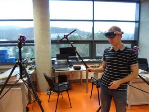
The aim of this study is to create the experimental data for real human movement and compare with the mathematical model. Vicon motion capture system is implemented for data acquisition. The Vicon system consists of 10 optical cameras (VERO Compact, economical, super-wide mobile camera @ 1.3/2.2 megapixels) providing the exact movements of markers placed on the body.
In order to calibrate the cameras, first, calibration process has been performed (Figure 2). This process designates to capture the system’s volume. The tracker can determine the lens properties, orientations and positions of all Vera cameras.
Figure 2. Calibration of the Vicon Motion Tracker
In this study, 18 markers are placed on the legs into the following positions:
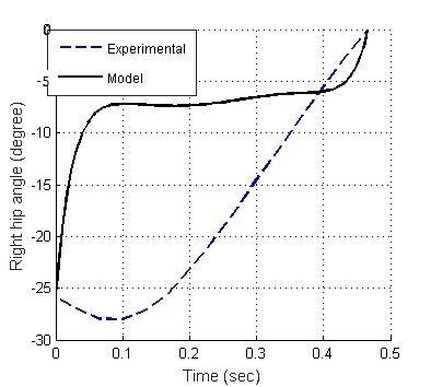
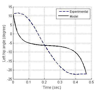
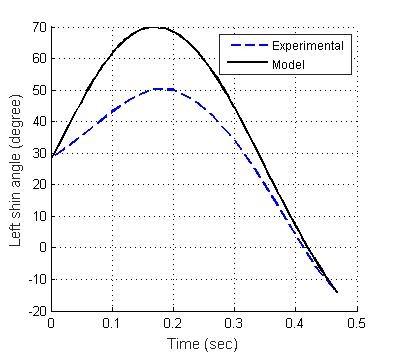
Figure 3 collections, show the mathematically modelling movement of a person based on the balanced energy (Eq.1 to 67) compared to the experimental data collected from Vicon.
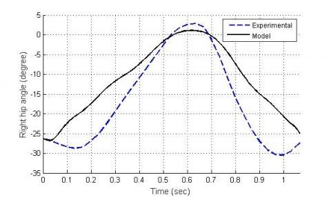
3.1 Right hip angles
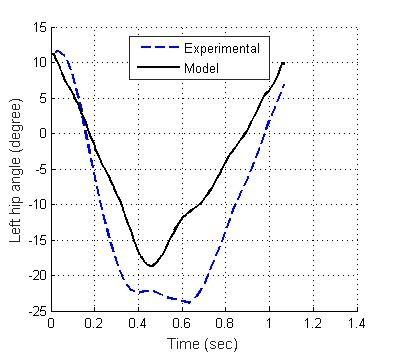
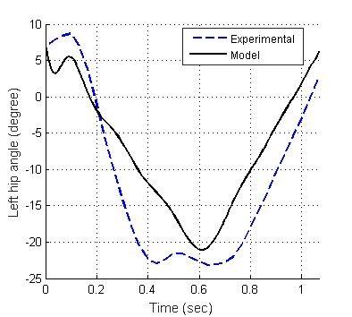
3.2 Left hip angles
3.3 Right shin angles
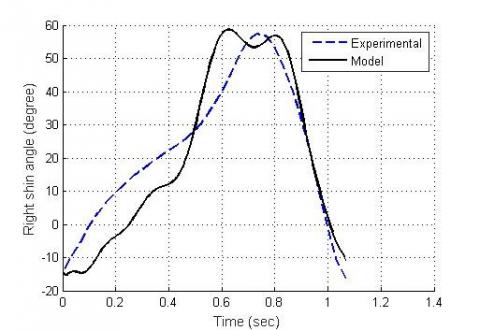
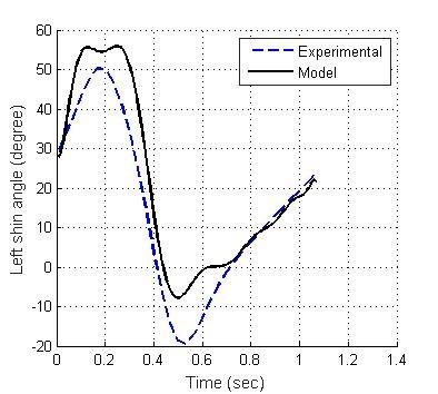
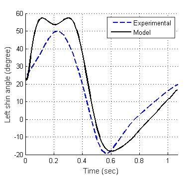
3.4 Left shin angles
Figure 3. Motions of model vs. experiment
It can be seen that the linearized model leads only to the correct end results. Only the dynamic motions of left shin angles in Figure 3.4 are coincided with the experimental data. All other mathematical model trajectories are not like the real motions because there is lack of controlled objective function and constraints. Therefore, in the next part, we develop MPC as the CNS to generate the optimal torques at each joint and subject to constraints to simulate the human gait motions.
The MPC algorithms for nonlinear (NMPC) are referred to [10]. The general expression for this linearized continuous time in state space is:
$\dot{x}(t)=\mathbb{A}_{C} x(t)+\mathbb{B}_{C} u(t)$ (68)
$y(t)=\mathbb{C}_{C} x(t)+\mathbb{D}_{C} u(t)$ (69)
where, x(t) represents the states, u(t) represents the inputs, y(t) represents the output, $\mathbb{A}_{C}$, $\mathbb{B}_{C}$, $\mathbb{C}_{C}$, $\mathbb{D}_{C}$ are the model state matrices in continuous time.
For computer calculation, the above continuous time system can be discretized (sampling interval T0= 0.01 sec) as:
$x(k+1)=\mathbb{A}_{D} x(k)+\mathbb{B}_{D} u(k)$ (70)
$y(k)=\mathbb{C}_{D} x(k)+\mathbb{D}_{D} u(k)$ (71)
where, x(k) represents the discrete states, u(k) represents the discrete inputs, y(k) represents the discrete output, $\mathbb{A}_{D}$, $\mathbb{B}_{D}$, $\mathbb{C}_{D}$, $\mathbb{D}_{D}$ are the state matrices in discrete form.
For simplification, we assign the state prediction, x(k), equal to the input prediction horizon, u(k), or $N_{x(k)}=N_{u(k)}=N$. Then, the objective function of this MPC is:
$J(x(k), u(k))=$$\frac{1}{2} \sum_{k=N_{0}}^{N-1}\left[x(k)^{T} Q x(k)+u(k)^{T} R u(k)\right]$$+\frac{1}{2} x(N)^{T} Q_{f} x(N)$ (72)
where, Q is the weighting matrix for the predicted states along the prediction horizon, R is the weighting matrix for the control inputs, and Qf is the weighting matrix for the final predicted states at the final time step. N is the horizon prediction length for both inputs and states.
Constraints for inputs are setup such as the maximum input torques and the limited joint angle at ankles, knees, hips:
$\min (u(k))<u(k)<\max (u(k))$ (73)
Similarly, constraints for states are also setup as:
$\min (x(k))<x(k)<\max (x(k))$ (74)
Example of constraints for hip of a healthy human is illustrated in Figure 4.
For the simplification, we set the horizon prediction length as N=50 for all simulations. A design MPC blocks in Matlab Simulink is developed and shown in Figure 5.
MPC designs and calculations are referred in the paper [9]. This MPC block is used as the internal model to control the external human plant model. The external human plant model is developed and presented in the next part.
Figure 4. Human hip constrains
The model of human plant is designed as five segments including shin, thigh on each side and a hard shell, which replaces the human body above the waist. The same pair of stop - two further segments can be added to the system. This simplification of the 5-link mechanism is taken since the movement of foot has little effect on the general movement of the low weight, and the calculation of the foot rotation considerably complicates our system. The blocks of human plant are developed in Matlab/Simulink and shown in Figure 5.
The inputs of this plant model are torques, which are supplied to actuators to set the rotation of the block links. The plant model has 5 bodies linked to each other through 4 rotational connections. This plant model describes the movement in one plane only. This simplification is permissible since movement in other planes significantly less. The human plant in Matlab Simulink is shown in Figure 6. These mechanical blocks are taken in the library of Matlab Simulink.
The above external plant model and the MPC internal model are used to verify the human CNS to perform the human motions. Simulation results are presented in the next part.
Figure 5. Human plant blocks
Figure 6. Human mechanical blocks
Human gait motions based on MPC are simulated and compared to the experimental data obtained by the Vicon motion capture cameras in ITMO University and partly in Technical University of Liberec. Mass units, moments of inertia, and the relative location of the centers of mass are estimated by the empirical equation (75) depending on the total mass (M) and the human height (H). The lengths of the links, the start and end positions are calculated with MPC controller.
$Y=B_{0}+B_{1} M+B_{2} H$ (75)
where, Y - segment mass, $B_{0}, B_{1}, B_{2}$ are coefficients given in Table 1.
Table 1. Coefficients of mass
|
Segment |
B0 |
B1 |
B2 |
|
Shin |
-1.592 |
0.0362 |
0.0121 |
|
Hip |
-2.649 |
0.1463 |
0.0137 |
|
Upper body |
10.3304 |
0.60064 |
0.04256 |
As referred in the paper [9], the first MPC is tested with zero terminals, x(N)=0. The MPC objective function in (72) becomes:
$J(x(0), u)=\frac{1}{2} \sum_{k=N_{0}}^{N-1}\left[x(k)^{T} Q x(k)+u(k)^{T} R u(k)\right]$ (76)
Simulation results of (76) are shown in Figure 7.
7.3 Sagittal plane right shin angle
7.4 Sagittal plane left shin angle
Figure 7. Model Predictive Controller with zero terminals
8.1 Sagittal plane right hip angle
8.2 Sagittal plane left hip angle
8.3 Sagittal plane right shin angle
8.4 Sagittal plane left shin angle
Figure 8. Model Predictive Controller with softened state constraints
MPC with zero terminals, x(N)=0, shows that, the models in Figure 7.1 and 7.3 do not follow the experimental motions. The model motions in Figure 7.2 and 7.4 have two peaks while the real experimental data has only one. Figures from 7.1 to 7.4 show that the mean of angle errors for the right and left hip is 6.2546° and 7.5277°, correspondingly. The mean of angle errors for right and left shin is 8.3327° and 7.9761°, correspondingly.
Next, another MPC controller with softened state constraints is developed:
$J(x(0), u)=$$\frac{1}{2} \sum_{k=N_{0}}^{N-1}\left[x(k)^{T} Q x(k)+u(k)^{T} R u(k)\right]+$$\sum_{k=N_{0}}^{N-1}\left[\varepsilon(k)^{T} M \varepsilon(k)+2 \mu(k)^{T} \varepsilon(k)\right]$ (77)
In (77), a penalty term of softened state constraints, $\sum_{k=N_{0}}^{N-1}\left[\varepsilon(\boldsymbol{k})^{T} \boldsymbol{M} \varepsilon(\boldsymbol{k})+2 \mu(\boldsymbol{k})^{T} \varepsilon(\boldsymbol{k})\right]$, is added with a positive definite and symmetric matrix, M, and usually large values, $\varepsilon(\boldsymbol{k})$. These terms help to penalize the violations of the state constraints, as $\mu(\boldsymbol{k})$ are the state violation values. Simulation results of MPC with softened constraints are shown in Figure 8.
Figure 8.1 to 8.4 show that the performances of the MPC with softened state constraints are better than the MPC with zero terminals. The mean of angle errors for the right and left hip is 4.8226° and 4.6601°, correspondingly. The mean of angle errors for the right and left shin is 3.95° and 4.145°. These values are much smaller than the MPC with zero terminals. Therefore, MPC with softened state constraints can be used well to predict the human gait motions. MPC with softened state constraints can also maintain the stability of the system and always keep the tracking errors at low levels.
The study has developed the mathematical model of human gait and MPCs as the CNS to simulate the human motions. Simulation results show that the system can generate the kinematic motions of normal persons. Tracking errors compared with experiments by VICON cameras, are not excessed 7%. The discrepancies can be caused by several reasons: Firstly, the model is highly simplified representation of the human body. Secondly, rotation occurs not only in the sagittal plane but also in the frontal and longitudinal planes. Thirdly, human movement must be considered in three separate intervals - singly, two-supporting and single support on the other foot, otherwise the inevitable errors due to non-equivalence of the support, can occur. Simulations show that the system with MPC can be used for study of different individual gaits for the diagnosis of diseases and for autonomous imaging of human gait. Further studies with different MPC algorithms and parameters by varying the weighting matrices, lengths of prediction, constraints are needed to perform in the next phase of this research, furthermore, applying non-linear based signal processing [21] combined with other innovative technologies like virtual and augmented reality [22] can extend the concept to the advanced phase.
The result was obtained through the financial support of the Ministry of Education, Youth and Sports of the Czech Republic and the European Union (European Structural and Investment Funds - Operational Programme Research, Development and Education) in the frames of the project “Modular platform for autonomous chassis of specialized electric vehicles for freight and equipment transportation”, Reg. No. CZ.02.1.01/0.0/0.0/16_025/0007293.
The authors also would like to thank TalTech University in Estonia and Saint Petersburg State University in Russia for the support of this collaborative research study. Without them this work would not be possible.
[1] Zhang, L.X., Wang, J.S., Wang, L., Wang, T. (2007). Experimental research on human gait measurement. Paper presented at the 2007 IEEE International Conference on Robotics and Biomimetics, ROBIO, pp. 167-171. https://doi.org/10.1109/ROBIO.2007.4522154
[2] Sminchbescu, C., Kanaujia, A., Li, Z.G., Metaxas, D. (2005). Conditional models for contextual human motion recognition. Paper presented at the Proceedings of the IEEE International Conference on Computer Vision, II pp. 1808-1815. https://doi.org/10.1109/ICCV.2005.59
[3] Aggarwal, J., Cai, Q. (1999). Human motion analysis: A review. Computer Vision and Image Understanding, 73(3): 428-440. https://doi.org/10.1006/cviu.1998.0744
[4] Perry, J., Davids, J.R. (2010). Gait analysis: Normal and pathological function. Journal of Sports Science & Medicine, 9(2): 353.
[5] Vergallo, P., Lay-Ekuakille, A., Angelillo, F., Gallo, I., Trabacca, A. (2015). Accuracy improvement in gait analysis measurements: Kinematic modeling. 2015 IEEE International Instrumentation and Measurement Technology Conference (I2MTC) Proceedings, Pisa, Italy. https://doi.org/10.1109/i2mtc.2015.7151587
[6] Luengas, L.A., Camargo, E., Sanchez, G. (2015). Modeling and simulation of normal and hemiparetic gait. Frontiers of Mechanical Engineering, 10(3): 233-241. https://doi.org/10.1007/s11465-015-0343-0
[7] Gill, T., Keller, J.M., Anderson, D.T., Luke, R.H. (2011). A system for change detection and human recognition in voxel space using the Microsoft Kinect sensor. 2011 IEEE Applied Imagery Pattern Recognition Workshop (AIPR), Washington, DC, USA. https://doi.org/10.1109/aipr.2011.6176347
[8] Sun J. (2015). Dynamic modeling of human gait using a model predictive control approach. PhD Dissertation Marquette University. https://epublications.marquette.edu/dissertations_mu/526/, accessed on 16 September 2020.
[9] Ren, L., Howard, D., Kenney, L. (2006). Computational models to synthesize human walking. Journal of Bionic Engineering, 3(3): 127-138. https://doi.org/10.1016/s1672-6529(06)60016-4
[10] Ren, L., Jones, R.K., Howard, D. (2007). Predictive modelling of human walking over a complete gait cycle. Journal of Biomechanics, 40(7): 1567-1574. https://doi.org/10.1016/j.jbiomech.2006.07.017
[11] Pontzer, H., Holloway, J.H., Raichlen, D.A., Lieberman, D.E. (2009). Control and function of arm swing in human walking and running. Journal of Experimental Biology, 212(4): 523-534. https://doi.org/10.1242/jeb.024927
[12] Mohammed, S., Samé, A., Oukhellou, L., Kong, K., Huo, W., Amirat, Y. (2016). Recognition of gait cycle phases using wearable sensors. Robotics and Autonomous Systems, 75: 50-59. https://doi.org/10.1016/j.robot.2014.10.012
[13] Minh, V.T., Afzulpurkar, N. (2008). A comparative study on computational schemes for nonlinear model predictive control. Asian Journal of Control, 8(4): 324-331. https://doi.org/10.1111/j.1934-6093.2006.tb00284.x
[14] Minh, V.T., Rashid, A.A. (2012). Modeling and model predictive control for hybrid electric vehicles. International Journal of Automotive Technology, 13: 477-485. https://doi.org/10.1007/s12239-012-0045-0
[15] Sun, J., Wu, S., Voglewede, P.A. (2018). Dynamic simulation of human gait model with predictive capability. Journal of Biomechanical Engineering, 140(3): 031008. https://doi.org/10.1115/1.4038739
[16] Falisse, A., Serrancolí, G., Dembia, C.L., Gillis, J., Jonkers, I., Groote, F.D. (2019). Rapid predictive simulations with complex musculoskeletal models suggest that diverse healthy and pathological human gaits can emerge from similar control strategies. Journal of The Royal Society Interface, 16(157): 20190402. https://doi.org/10.1098/rsif.2019.0402
[17] Pitto, L., Kainz, H., Falisse, A., Wesseling, M., Rossom, S.V., Hoang, H., Jonkers, I. (2019). SimCP: A simulation platform to predict gait performance following orthopedic intervention in children with cerebral palsy. Frontiers in Neurorobotics, 13: 54. https://doi.org/10.3389/fnbot.2019.00054
[18] Schreiber, C., Moissenet, F. (2019). A multimodal dataset of human gait at different walking speeds established on injury-free adult participants. Scientific Data, 6: 111. https://doi.org/10.1038/s41597-019-0124-4
[19] Minh, V.T., Afzulpurkar, N. (2008). A comparative study on computational schemes for nonlinear model predictive control. Asian Journal of Control, 8(4): 324-331. https://doi.org/10.1111/j.1934-6093.2006.tb00284.x
[20] Xu, Y.P. (2017). A study of hydropower generation process control based on fuzzy control theory. European Journal of Electrical Engineering, 19(3-4): 167-179. https://doi.org/10.3166/EJEE.19.167–179
[21] Moezzi, R., Hlava, J., Vu, T.M. (2019). Implementation of X-parameters principle for non-linear vibroacoustic membrane using two-port measurement. Traitement du Signal, 366(4): 297-301. https://doi.org/10.18280/ts.360401
[22] Moezzi, R., Krcmarik, D., Bahri, H., Hlava, J. (2019). Autonomous vehicle control based on HoloLens technology and raspberry pi platform: An educational perspective. Paper presented at the IFAC-Papers Online, 52(27): 80-85. https://doi.org/10.1016/j.ifacol.2019.12.737