Chunxiao Chen* | Liyun Wei | Zhiya Chen | Chuijiang Guo
OPEN ACCESS
The completion of passenger-dedicated lines (PDLs) has released the transport capacity of many existing railways, making room for railway freight transport. To make full use of the released capacity, this paper puts forward an integer linear programming model based on the linear correlation between the number of trains and the demand increment, and solves the model with IBM ILOG CPLEX Optimization Studio 12.4. The proposed model was successfully applied to prepare a suitable operation plan of two types of freight block trains (FBTs) in a railway network with multiple routes and nodes. To further increase the transport profit, two only adjustable parameters, namely, the capacity of railway section and the number of trains, were subjected to sensitivity analysis. Through the analysis, the author determined which railway sections should expand their capacities and which way stations should increase the number of FBTs.
passenger-dedicated lines (PDLs), freight block trains (FBTs), operation planning, sensitivity analysis
China boasts a vast territory with uneven distribution of resources. Therefore, railway has become the primary way to transport goods and passengers, exerting great impacts on national economy and people’s livelihood. In recent years, the transport demand of both goods and passengers is soaring in the transport corridors between major Chinese cities. However, many trunk railways are almost saturated [1]. The lack of capacity has limited the transport of goods other than those essential to livelihood, such as coal, ore and grain. The railway freight transport is further restricted by the fact that passenger trains have superior track occupancy rights over freight trains. Therefore, the traditional railway transport services (e.g. through trains, transit trains and district trains) are not suitable for transferring goods with high demand of timeliness and high additional value.
The plight of railway freight transport is expected to lighten with the emerging passenger-dedicated lines (PDLs) across China. Some passenger trains have been relocated from existing railways to the PDLs, releasing a great amount of route capacity for freight transport. Statistics show that the operation of four PDLs (Jinan–Qingdao, Beijing–Tianjin, Wuhan–Guangzhou and Shanghai–Ningbo) alone released a route capacity of 230 million ton per year [2]. According to official plans, China will complete a “Four Vertical and Four Horizontal” network of the PDLs, releasing even more route capacity of existing railways. To fully utilize the released capacity, it is necessary to optimize the trainload service for railway freight transport, including but not limited to the departure and terminal stations, the number of cars, and the departure and arrival times.
The optimization of trainload service must consider the current trends in transport demand of China’s railways, and refer to the relevant practices in developed countries. China has now entered a “new normal” of economic development. The once-dominant primary industry is being overtaken by secondary and tertiary industries. Under this new normal, the transport demand of agricultural goods like fertilizer and gain is falling, while that of industrial goods with high added value has shot up. In many developed countries, the latest freight railways have common features like heavy haul, high level of informatization, combined transport and centralized scheduling, creating a mature operation network for freight block trains (FBTs) [3].
To fully utilize the released route capacity, this paper puts forward an FBT operation model based on the linear correlation between the number of trains and the demand increment. The model parameters like the number of trains, operation frequency, maximum load per train were defined and calibrated based on a railway network with multiple routes and nodes [4]. Next, the model was solved with IBM ILOG CPLEX Optimization Studio 12.4, and verified through an example railway network. Finally, the author conducted a sensitivity analysis on the capacity of railway section and the number of trains to future increase the profit of railway transport enterprise.
The FBTs and fast freight trains are two new types of railway freight trains. The FBTs are fixed in five aspects, namely, time, route, freight, stations and number of cars, while fast freight trains are not fixed in these aspects. Besides, the FBTs operate at three levels of speed (i.e. ultra-high speed, high speed, and normal speed), while the fast freight trains can reach a maximum speed of 120km/h. Comparatively, the FBTs are more suitable for the transport of light goods with high additional value.
Many Chinese and foreign scholars have designed operation plans for railway freight trains and similar transport vehicles. For example, Assad [5] proposed several combinatorial optimization models that tackle train routing and marshalling based on network flow. Crainic and Rousseau [6] established a mixed integer programming (MIP) model to rationalize resource allocation and minimize the operating cost of transport enterprises. To minimize the operation time, Martinelli and Teng [7] built a nonlinear integer programming model for a railway operation plan, and presented a neural network (NN) to solve the model. Gorman [8] designed an operating-plan model (OPM) for the Atchison, Topeka and Santa Fe (ATSF) Railway Company, and solved the model with a hybrid algorithm coupling genetic search and Tabu search. With the aid of the OPM, the railway company slashed its operating cost by 4~6%. Targeting the scheduling of trains and containers with due dates, Yano and Newman [9] formulated an optimization model and an algorithm to minimize the transport cost and the holding cost. Considering the optimal fleet size, route and schedule, Lai and Lo [10] put forward a ferry network design strategy for both direct and multi-stop services. Jeong et al. [11] included the time and cost of freight transport into Aijang’s models. Ceselli et al. [12] prepared three operation plans to optimize the routing, scheduling, locomotive assignment and marshalling of freight trains. In view of pricing policy and network capacity, Crevier et al. [13] constructed a bilevel model for the operation plan of railway freight transport, and then created a solving algorithm based on the branch-and-bound (BB) algorithm. Zhang and Yan [14] aimed to optimize the operation plan for fast freight trains based on transport volume, frequency and transit time, set up an integer programming model for the maximal freight demand, and applied to model to assign trains to candidate routes. Xiao et al. [15,16] used single- and two-block trains to solve the marshalling problem of the FBTs in China.
The above studies provide references for the design and optimization of FBT operation plan. However, the models of most studies only consider the situation in the current year and assume that the demand for railway freight is static, ignoring the demand fluctuation induced by the train operations. This paper aims to solve the two defects through the construction of an integer linear programming model.
3.1 Hypotheses
The following hypotheses were put forward before creating the new FBT operation plan:
Hypothesis 1. The carrier mode (i.e. locomotive and car(s)) is not considered in our model.
Hypothesis 2. The impacts of operations on the FBT at way stations (nodes) in the railway network are negligible.
Hypothesis 3. The attributes of the FBT are fixed, namely, number of cars, type of goods, to name but a few.
Hypothesis 4. The railways are all electrified double track railways.
Hypothesis 5. With the increasing operating frequency of the FBTs, the freight demand will have a rapid linear growth.
Hypothesis 6. The FBTs have superior track occupancy rights over ordinary freight trains.
3.2 Symbols
For simplicity, the following symbols were defined as given conditions.
The following symbols are defined. These symbols are regarded as given conditions.
(a) Sets
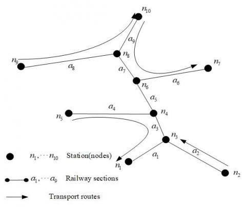
(1) As shown in Figure 1, the railway network is denoted as G=(N,A), where, N is the set of n∈N way stations (nodes) in the network and A is the set of a∈A railway sections. The railway section refers to the segment of the railway between two adjacent way stations.
Figure 1. An example of railway network
(2) In the railway network, OD is the set of od∈OD transport routes, where, O is the set of o∈O origins (departure stations) and D is the set of d∈D destinations (terminal stations).
(3) T is the set of t∈T years. Here, T only covers three years, because this paper only focuses on the transport profit in the short term.
(4) K is the set of k∈K types of FBTs. Here, two types of FBTs are discussed, namely, high-speed freight block trains (HFBTs) and normal-speed freight block trains (NFBTs).
(b) Coefficients
(1) $S _ { k } ^ { o d }$ is the income of transporting one unit of goods on route od by a type k FBT, including the freight charge, the surcharge for using electrified railways, and the surcharge for railway construction fund. If the FBT is an HFBT, then $S _ { k } ^ { o d }$ also contains an extra express fee.
(2) $c _ { k } ^ { o d }$ is the operating cost of a type k FBT from the origin o to destination d. This cost consists of departure fee, arrival fee, railway occupancy fee, locomotive traction fee, etc.
(3) αk is the deduction coefficient of a type k FBT.
(4) $Q_ { t } ^ { o d }$ is the freight demand on route od in year t.
(5) $q_ { k } ^ { o d }$ is the freight demand increment on route od in the next year, for each additional type k FBT.
(6) $Cap_ { t } ^ { a }$ is the capacity of railway section a in year t.
(7) $R_ { k t } ^ { o }$is limit on the number of type k FBTs in origin o in year t.
(8) Bk is the maximum load of a type k FBT.
(c) Decision variables
(1) $\varphi _ { akt } ^ { o d }$ is the relationship between route od and railway section a. If railway section $a$ belongs to route od, $\varphi _ { akt } ^ { o d }$ equals one; otherwise, $\varphi _ { akt } ^ { o d }$ equals zero.
(2) $F _ { k t } ^ { o d }$ is the total load of goods transported by a type k FBT on route od in year t. This decision variable can only take integer values.
(3) $P _ { k t } ^ { o d }$ is the number of type k FBTs on route od in year t. This decision variable can only take integer values.
3.3 Mathematical model
Our model aims to maximize the transport profit in the short term. Hence, the objective function can be defined as:
$\max ( S - C )$
$\left\{ \begin{array} { l } { S = \sum _ { o \in O } \sum _ { d \in D } \sum _ { t \in T } \sum _ { k \in K } s _ { k } ^ { o d } f _ { k t } ^ { o d } } \\ { C = \sum _ { o \in O}\sum _ { d \in D } \sum _ { t \in T } \sum _ { k \in K } c _ { k } ^ { o d } P _ { k t } ^ { o d } } \end{array} \right.$ (1)
where, S is the total income; C is the total cost. The difference between S and C is the transport profit of the railway network. Our model is subjected to six constraints: the train flow in each railway section must be smaller than or equal to the capacity of that section; the number of type k FBTs operating in origin o in year t should not surpass the limit; the freight demand on each route in the current year should be increased, only if the number of FBTs on that route is within the limit in the previous year; the total load of goods on each transport route should not exceed the maximum load of all FBTs operating on that route; the total load of goods on each transport route should equal the total freight demand on that route; the decision variables should be satisfy logic restriction. The formulas of the six constraints are presented in turn:
$\sum _ { o \in D } \sum _ { d \in D } \sum _ { k \in K } P _ { k t } ^ { o d } \varphi _ { a k t } ^ { o d } \alpha _ { k } \leq \operatorname { Cap } _ { a } ^ { t } \quad \forall t \in T , a \in A$ (2)
$\sum _ { d \in D } P _ { k t } ^ { o d } \leq \varphi _ { k t } ^ { o } \quad \forall t \in T , k \in K , o \in O$ (3)
$Q _ { t } ^ { o d } = Q _ { 0 } ^ { o d } + \sum _ { t - 1 } \sum _ { k \in K } q _ { k } ^ { o d } P _ { k t } ^ { o d } \quad \forall t \in T , o \in O , d \in D$ (4)
$F _ { k t } ^ { o d } \leq B _ { k } P _ { k t } ^ { o d } \quad \forall t \in T , k \in K , o \in O , d \in D$ (5)
$\sum _ { k \in K } F _ { k t } ^ { o d } = Q _ { t } ^ { o d } \quad \forall t \in T , o \in O , d \in D$ (6)
$P _ { k t } ^ { o d } \in Z ^ { + } F _ { k t } ^ { o d } \in Z ^ { + } \quad \forall t \in T , k \in K , o \in O , d \in D$
$\varphi _ { a k t } ^ { o d } \in ( 0,1 ) \quad \forall t \in T , k \in K , o \in O , d \in D , a \in A$ (7)
Through the above analysis, the design of a practical operation plan was transformed into a capacity constraint problem of a railway network with multiple routes and nodes. The established integer linear programming model can be solved by various mature algorithms or software toolboxes, ranging from the BB algorithm, the cutting-plane algorithm, heuristic algorithms (e.g. genetic algorithm (GA) and simulated annealing (SA) algorithm), MATLAB, LINGO to CPLEX [17]. In this paper, the established model is solved by the professional optimization software: IBM ILOG CPLEX Optimization Studio 12.4.
4.1 Background
With more and more PDLs entering operation, a large proportion of Chinese passengers choose to travel by high-speed rail. As a result, many existing railways, which used to be fully occupied, suddenly become unsaturated [18, 19]. The released capacity allows railway transport enterprises to optimize the trainload services for freight transport.
According to a recent survey on railway transport market, the goods with high added value only accounted for a small portion of freight transport in Chinese railways. Therefore, the traditional freight trains often operate at low frequencies to transfer bulk goods, which belong to the same or similar categories. However, the transport demand for high added-value goods has rocketed up in recent years, calling for brand-new operation plans of freight trains. That is why this paper aims to develop an operation plan of FBTs for high added-value goods.
4.2 Parameter calibration
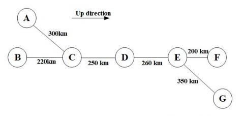
Figure 2 displays a typical railway network, which contains seven ways stations (nodes) and four origins/terminals. The distance between adjacent stations, i.e. the length of railway sections, ranges from 200 to 350 km. In each railway section, two types of FBTs are in operation, namely, the HFBT and the NFBT. Every FBT has the same formation: a locomotive and fifty P65 box cars. According to the technical data of P65 box car and the Guidelines issued by Chinese Ministry of Transport, the maximum loads of the HFBT and the NFBT were 2,250 and 2,900 ton/train, respectively. The deduction coefficients of the two types of FBTs were selected from the allowable range of 1.2~3.0: 2.5 for each HFBT and 1 for each NFBT.
Figure 2. A typical railway network
As discussed above, high added-value goods are the target of the operation planning of the FBTs. This kind of goods raises a high requirement on the service level of the FBTs. The operation frequency is a key influencing factor of the service level. In general, the higher the operation frequency, the better the realization of potential freight demand. It is assumed that an additional HFBT can increase the freight demand in the next year on the current route by 300 tons, while an additional NFBT can only increase that demand by 100 tons. The original freight demand of the railway network is described in Table 1.
Table 1. Original freight demand of the railway network
|
No. |
Transport route |
Original freight demand (Million tons) |
|
1 |
A→E |
110 |
|
2 |
A→F |
120 |
|
3 |
B→D |
100 |
|
4 |
B→G |
180 |
|
5 |
C→G |
140 |
|
6 |
D→A |
100 |
|
7 |
D→F |
90 |
|
8 |
E→B |
150 |
|
9 |
F→B |
200 |
|
10 |
F→C |
120 |
|
11 |
G→A |
110 |
|
12 |
G→D |
130 |
The high added-value goods fall into various categories, namely, food, toys, stationeries and textiles. These goods are often supplied in small batches. The volume of each batch cannot fill up a box car. Therefore, the transport enterprise needs to charge the shipper extra fees in addition to the base prices (base price 1: RMB 0.0235 yuan/kg·km; base price 2: RMB 0.00012 yuan/kg·km), including the surcharge for using electrified railways (RMB 000033 yuan/ kg·km), and the surcharge for railway construction fund (RMB 0.000012 yuan/kg·km). If the FBT is an HFBT, then the total freight charge should be floated by 30%. The reduction in human and material resources should also be considered to determine the income of the transport enterprise. Meanwhile, the operation cost of an FBT consists of departure fee, arrival fee, railway occupancy fee, locomotive traction fee, etc. The transport income and cost on each route are listed in Table 2 below.
Table 2. Transport income and cost on each route
|
Transport route |
Type of train |
Income (RMB yuan/ton) |
Cost (RMB yuan/train) |
|
A→E |
HFBTs |
204.295 |
202380 |
|
NFBTs |
157.15 |
145370 |
|
|
A→F |
HFBTs |
247.195 |
221980 |
|
NFBTs |
190.15 |
160770 |
|
|
B→D |
HFBTs |
131.365 |
169060 |
|
NFBTs |
101.05 |
119190 |
|
|
B→G |
HFBTs |
262.21 |
228840 |
|
NFBTs |
201.7 |
166160 |
|
|
C→G |
HFBTs |
215.02 |
207280 |
|
NFBTs |
165.4 |
149220 |
|
|
D→A |
HFBTs |
148.525 |
176900 |
|
NFBTs |
114.25 |
125350 |
|
|
D→F |
HFBTs |
129.22 |
168080 |
|
NFBTs |
99.4 |
118420 |
|
|
E→B |
HFBTs |
187.135 |
194540 |
|
NFBTs |
142.95 |
139210 |
|
|
F→B |
HFBTs |
230.035 |
214140 |
|
NFBTs |
176.95 |
154610 |
|
|
F→C |
HFBTs |
182.845 |
192580 |
|
NFBTs |
140.65 |
137670 |
|
|
G→A |
HFBTs |
279.37 |
236680 |
|
NFBTs |
214.9 |
172320 |
|
|
G→D |
HFBTs |
161.395 |
182780 |
|
NFBTs |
124.15 |
129970 |
Table 3. Capacity limit for each railway section
|
Railway section (up direction) |
Capacity limit (train) |
Railway section (up direction) |
Capacity limit (train) |
|
A→C |
8 |
F→E |
10 |
|
B→C |
10 |
G→E |
10 |
|
C→D |
15 |
E→D |
18 |
|
D→E |
16 |
D→C |
19 |
|
E→F |
7 |
C→B |
8 |
|
E→G |
6 |
C→A |
7 |
Some way stations have strict requirements on the number of operating FBTs, especially HFBTs, due to the locomotive operation and station capacity. Table 4 describes the limits on the number of FBTs in each way station.
Table 4. The limits on the number of FBTs in each way station
|
Way station |
Limits on the number of FBTs (trains/day) |
|
|
HFBT |
NFBT |
|
|
A |
2 |
2 |
|
B |
2 |
Unlimited |
|
C |
1 |
1 |
|
D |
1 |
Unlimited |
|
E |
1 |
2 |
|
F |
3 |
Unlimited |
|
G |
2 |
3 |
4.3 Simulation results
The integer linear programming problem was solved on IBM ILOG CPLEX Optimization Studio 12.4, using the calibrated parameters. The optimal solution RMB 5,718,449,794 was obtained in 31s. It is the sum of the annual incomes in the three years. Table 5 records of the number of each type of FBTs operating in the network every year.
Table 5. The number of each type of FBTs operating in the network every year
|
Transport route |
Year |
Number of FBTs (trains/year) |
|
|
HFBT |
NFBT |
||
|
A→E
|
1 |
199 |
225 |
|
2 |
125 |
311 |
|
|
3 |
46 |
396 |
|
|
A→F
|
1 |
531 |
2 |
|
2 |
603 |
1 |
|
|
3 |
684 |
1 |
|
|
B→D |
1 |
250 |
151 |
|
2 |
339 |
113 |
|
|
3 |
0 |
415 |
|
|
B→G
|
1 |
478 |
250 |
|
2 |
389 |
377 |
|
|
3 |
300 |
500 |
|
|
C→G |
1 |
152 |
365 |
|
2 |
191 |
363 |
|
|
3 |
230 |
365 |
|
|
D→A
|
1 |
362 |
64 |
|
2 |
363 |
103 |
|
|
3 |
6 |
421 |
|
|
D→F
|
1 |
2 |
309 |
|
2 |
2 |
320 |
|
|
3 |
2 |
331 |
|
|
E→B
|
1 |
364 |
235 |
|
2 |
365 |
280 |
|
|
3 |
2 |
609 |
|
|
F→B |
1 |
626 |
204 |
|
2 |
560 |
327 |
|
|
3 |
853 |
169 |
|
|
F→C
|
1 |
469 |
50 |
|
2 |
535 |
49 |
|
|
3 |
240 |
335 |
|
|
G→A |
1 |
489 |
0 |
|
2 |
553 |
1 |
|
|
3 |
628 |
0 |
|
|
G→D |
1 |
241 |
262 |
|
2 |
177 |
345 |
|
|
3 |
96 |
438 |
|
The operation plan for trains on each route can be seen clearly on the above table. For instance, 626 HFBTs and 204 NFBTs operated on route F→B in the first year. Note that route D→F only had 2 HFBTs while route G→A had almost no NFBT through the three years. This is the result of the capacity of the railway sections and the limit on the number of FBTs.
The most profitable operation plan can be obtained easily based on the known information. However, the transport enterprises may want to further adjust the plan and earn more profit. The only adjustable parameters are the capacity of railway section and the number of trains. The other parameters, such as the transport income, transport cost and maximum load of trains, are fixed values and not likely to change in the short term, if no technical breakthrough is made soon. Hence, the next step is to analyse how the capacity of railway section and the number of trains affect the transport profit.
5.1 Capacity of railway section
The capacity of railway section has a great impact on train operations. A railway section with high capacity allows more trains to operate, thus increasing the transport income. To disclose how this capacity impacts transport profit, the capacity of railway sections in our example were increased in the following manner: each time, the capacity of one railway section was increased by 5, without changing that of any other section. The analysis results are shown in Table 6 below.
Table 6. The transport profits after adjusting the capacity of railway section
|
Adjusted railway section |
Transport profit (RMB yuan) |
Profit increment (RMB yuan) |
|
A→C |
5,718,449,794 |
0 |
|
B→C |
5,718,557,670 |
107,876 |
|
C→D |
5,718,569,899 |
120,105 |
|
D→E |
5,718,561,486 |
111,692 |
|
E→F |
5,718,460,789 |
10,995 |
|
E→G |
5,764,293,358 |
45,843,564 |
|
F→E |
5,718,574,065 |
124,271 |
|
G→E |
5,718,449,794 |
0 |
|
E→D |
5,718,482,242 |
32,448 |
|
D→C |
5,718,484,294 |
34,500 |
|
C→B |
5,744,825,442 |
26,375,648 |
|
C→A |
5,718,569,899 |
120,105 |
As shown in Table 6, the transport profits changed by different degrees through the adjustment, ranging from 0 to RMB 45,843,564 yuan. For example, after the capacity of railway section A→C increased from 8 to 13, the transport profit of the network remained the same as the original value. This means the capacity of railway section A→C already fully satisfy the transport demand in the initial condition, eliminating the need for capacity expansion. Similar results were observed in railway section G→E. By contrast, the capacity growth in the other sections more or less boosted the profit, especially in C→B and E→G. These two sections should be focused in capacity adjustment, for they contribute the most to the network profit. Comparatively, the capacity growth in E→G can bring more profit than that in C→B.
5.2 Number of trains
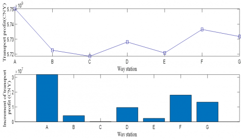
The transport profit also has something to do with the number of trains operating in each station. In way stations, the limit on FBTs mainly targets the HFBTs. To reveal the effects of the number of trains on transport profit, the number of HFBTs was increased in the following manner: one more HFBT was deployed per day in one of the seven ways stations, without changing the number of HFBTs in any other way station. The analysis results are illustrated in Figure 3 below.
Figure 3. The level and increment of transport profit after adjusting the number of HFBTs
From Figure 3, it can be seen that the increment of transport profit fell between RMB 132,420 yuan and RMB 31,867,325 yuan. The most marked increment was observed in station E. Thus, the transport enterprise should deploy more HFBTs in this station to maximize the profit.
The traditional methods for FBT operation planning basically overlook the demand fluctuation induced by the train operations. To make up for the gap, this paper sets up an integer linear programming model for FBT operation planning. The model construction fully considers the linear relationship between the number of trains and the demand increment under the operation plan. Then, the model was solved by IBM ILOG CPLEX Optimization Studio 12.4 and applied to prepare a suitable operation plan of two types of FBTs in a railway network. Finally, the capacity of railway section and the number of trains were subjected to sensitivity analysis, revealing which railway sections should expand their capacities and increase the number of FBTs. The research findings help Chinese railway transport enterprises to make full use of the newly released capacity of existing railways. The future research will explore the planning of train operations, under the premise that the demand increment increases nonlinearly with the number of trains, and will also discuss the operation plan of another type of freight trains.
This work was supported by the National Natural Science Foundation of China (Grant Number 71401182), Philosophy and Social Foundation of Hunan (Grant Number 2018YBG021), Educational Commission of Hunan Province of China (Grant Number 18C1522).
[1] Lin, B.L., Wang, Z.M., Ji, L.J., Tian, Y.M., Zhou, G.Q. (2012). Optimizing the freight train connection service network of a large-scale rail system. Transportation Research, Part B: Methodological, 46(5): 649-667. https://doi.org/10.1016/j.trb.2011.12.003
[2] Yin, M., Bertolini, L., Duan, J. (2015). The effects of the high-speed railway on urban development: international experience and potential implications for China. Progress in Planning, 98: 1-52. https://doi.org/10.1016/j.progress.2013.11.001
[3] Yang, L., Gao, Z., Li, K. (2011). Railway freight transportation planning with mixed uncertainty of randomness and fuzziness. Applied Soft Computing Journal, 11(1): 778-792. https://doi.org/10.1016/j.asoc.2009.12.039
[4] Huang, Z., Niu, H. (2012). The mode of combined multi-speed freight trains under separation of passenger and freight transport. Procedia-Social and Behavioral Sciences, 43: 709-717. https://doi.org/10.1016/j.sbspro.2012.04.144
[5] Assad, A.A. (1980). Modelling of rail networks: toward a routing/makeup model. Transportation Research Part B: Methodological, 14(1-2): 101-114. https://doi.org/10.1016/0191-2615(80)90036-3
[6] Crainic, T., Rousseau, F.M. (1984). A tactical planning model for rail freight transportation. Transportation Science, 18(2): 165-184. https://doi.org/10.2307/25768127
[7] Martinelli, D.R., Teng, H. (1996). Optimization of railway operations using neural networks. Transportation Research Part C (Emerging Technologies), 4(1): 33-49. https://doi.org/10.1016/0968-090X(95)00019-F
[8] Gorman, M.F. (1998). Santa Fe Railway uses an operating-plan model to improve its service design. Interfaces, 28(4): 1-12. https://doi.org/10.2307/25062392
[9] Yano, C.A., Newman, A.M. (2001). Scheduling trains and containers with due dates and dynamic arrivals. Transportation Science, 35(2): 181-191. https://doi.org/10.1287/trsc.35.2.181.10132
[10] Lai, M.F., Lo, H.K. (2004). Ferry service network design: optimal fleet size, routing, and scheduling. Transportation Research, Part A (Policy and Practice), 38(4): 305-328. https://doi.org/10.1016/j.tra.2003.08.003
[11] Jeong, S.J., Lee, C.G., Bookbinder, J.H. (2007). The European freight railway system as a hub-and-spoke network. Transportation Research Part A: Policy and Practice, 41(6): 523-536. https://doi.org/10.1016/j.tra.2006.11.005
[12] Ceselli, A., Gatto, M., Lübbecke, Marco E., Nunkesser, M., Schilling, H. (2008). Optimizing the cargo express service of swiss federal railways. Transportation Science, 42(4): 450-465. https://doi.org/10.1287/trsc.1080.0246
[13] Crevier, B., Cordeau, J.F., Savard, G. (2012). Integrated operations planning and revenue management for rail freight transportation. Transportation Research, Part B: Methodological, 46(1): 100-119. https://doi.org/10.1016/j.trb.2011.09.002
[14] Zhang, Y., Yan, Y. (2014). An operation optimization for express freight trains based on shipper demands. Discrete Dynamics in Nature and Society, 2014(2): 1-8. https://doi.org/10.1155/2014/232890
[15] Xiao, J., Lin, B. (2016). Comprehensive optimization of the one-block and two-block train formation plan. Journal of Rail Transport Planning & Management, 6(3): 218-236. https://doi.org/10.1016/j.jrtpm.2016.09.002
[16] Xiao, J., Lin, B., Wang, J. (2018). Solving the train formation plan network problem of the single-block train and two-block train using a hybrid algorithm of genetic algorithm and tabu search. Transportation Research Part C: Emerging Technologies, 86: 124-146. https://doi.org/10.1016/j.trc.2017.10.006
[17] Guastaroba, G., Savelsbergh, M., Speranzaa, M.G. (2017). Adaptive kernel search: A heuristic for solving mixed integer linear programs. European Journal of Operational Research, 263(3): 789-804. https://doi.org/10.1016/j.ejor.2017.06.005
[18] Xu, S., Gang, Z., Bo, A., Zhong, Z. (2016). A survey on high-speed railway communications. Computer Communications, 86: 12-28. https://doi.org/10.1016/j.comcom.2016.04.003
[19] Harrod, S.S. (2012). A tutorial on fundamental model structures for railway timetable optimization. Surveys in Operations Research and Management Science, 17(2): 85-96. https://doi.org/10.1016/j.sorms.2012.08.002