Abdeldjalil Ledmi*![]() | Makhlouf Ledmi
| Makhlouf Ledmi![]() | Mohammed El Habib Souidi
| Mohammed El Habib Souidi![]() | Hichem Haouassi
| Hichem Haouassi![]() | Dalal Bardou
| Dalal Bardou![]()
© 2024 The authors. This article is published by IIETA and is licensed under the CC BY 4.0 license (http://creativecommons.org/licenses/by/4.0/).
OPEN ACCESS
Task scheduling in cloud computing represents a pivotal challenge, necessitating the efficient allocation of computing tasks to available resources. This challenge is crucial in diverse sectors such as e-commerce, e-learning, and e-health, and is compounded by the heterogeneity of tasks and resources, fluctuating demands, and the need to optimize multiple objectives like Makespan, resource utilization, and throughput. In the quest to resolve these complexities, meta-heuristic algorithms inspired by natural phenomena have gained prominence. Among them, the Tuna Swarm Optimization (TSO) algorithm stands out for its proficient ability to navigate and exploit the search space effectively. This paper introduces a novel algorithm, the Discrete Tuna Swarm Optimization for Task Scheduling (DTSO-TS), derived from the TSO algorithm. DTSO-TS algorithm's goal is to efficiently distribute tasks among virtual machines, balance workloads and improve resource utilization to minimize Makespan while increasing throughput. A fitness function provides optimal solutions to this goal. Creates a swarm before evaluating and refining solutions which have proven their worth. By contrasting it with well-known scheduling algorithms such as Ant-Colony-Based, Particle Swarm Optimisation, Genetic Algorithm, First Come First Serve, Round Robin, and Shortest Job First, we may evaluate DTSO-TS's effectiveness. According to the comparison results, DTSO-TS is the best option for scheduling tasks in cloud computing contexts.
cloud computing, task scheduling, Discrete Tuna Swarm Optimization (DTSO), load balancing, performance evaluation, makespan, throughput time, average waiting time
Cloud computing, often recognized as an innovative computer model, enables organizations to access an on-demand pool of computing resources while only paying for what they use [1]. This model offers many benefits, such as instant resource availability and cost efficiency. However, one major challenge encountered by organizations today is task scheduling: the efficient allocation of resources to tasks that is termed task allocation. Task scheduling in cloud computing, essential to efficiently allocating computing resources [2, 3], strives to maximize Makespan, energy consumption and resource utilization metrics. Due to cloud environments' dynamic environments and multiple possible task/resource allocation scenarios, its difficulty makes this challenge an NP-hard problem [4], which must be met efficiently if optimal performance metrics are to be attained.
Recently, studies have found evidence that inefficient task scheduling in cloud computing can negatively impact performance efficiency and drastically increase resource use [5]. The suboptimal allocation of tasks using traditional scheduling strategies such as First Come First Served (FCFS), Round Robin (RR) and Shortest Job First (SJF) has proven insufficient for dynamic cloud environments [6]. These linear optimization approaches often lack scalability and fail to deliver satisfactory results. Metaheuristic algorithms are becoming widely sought after due to their ability to quickly search complex spaces for near-optimal solutions within realistic timeframes [7], including the Bat Algorithm (BA) [8], Grey Wolf Optimization (GWO) [9], Ant Colony Optimization (ACO) [10], Dragonfly Algorithm (DA) [11], Genetic Algorithm (GA) [12], Artificial Bee Colony (ABC) [13], and Particle Swarm Optimization (PSO) [14]. Nonetheless, some metaheuristics may require high computational complexity or exhibit poor performance.
This study introduces the DTSO-TS algorithm based on tuna swarm intelligence systems designed explicitly for discrete task-scheduling aimed at attaining optimal metrics like Makespan Resource utilization. Throughput response time average waiting period with an emphasis placed on Cloud Computing settings.
The performance of the DTSO-TS algorithm was evaluated in simulations using the CloudSim simulator [15]. The AC-based algorithm [16], PSO [17], GA-based load balancing [18], FCFS, RR and SJF were established scheduling algorithms used for comparison purposes. Evaluations were focused on several metrics such as Makespan, resource utilization, response time throughput time average waiting times. Results showed that the DTSO-TS algorithm outperformed its counterparts by achieving higher throughput times while optimizing Makespan and maintaining low response times and average waiting times. This work introduces the DTSO-TS algorithm, filling a crucial research gap in efficient task scheduling methods for cloud computing environments. Deployment of this algorithm in such environments aims to produce significant gains across various performance metrics; its efficacy against competing scheduling algorithms was tested through simulations to provide an evaluation.
To facilitate comprehension, this study employs various performance metrics that are commonly utilized when assessing task scheduling algorithms in cloud computing. These performance metrics include:
The paper's organization includes Section 2 offering insights into literature review on cloud computing task schedules outlining research gaps pertinent towards motivations behind carrying out our work. This article also discusses TSO algorithm in Section 3 alongside problem formulation regarding DTSO-TS technique described extensively under Section 4. In Sections 5-6, the implementation design choices combined with simulation results & evaluations' coverage involving existing approach comparisons precedes concluding remarks highlighting contributions made whilst discussing future directions impacting further related studies.
Task scheduling is a crucial element of cloud computing that plays an important role in performance and efficiency. This process involves assigning tasks to available resources like virtual machines or physical servers, while considering various constraints such as minimizing execution time, maximizing resource utilization and reducing energy consumption.
To address these complexities, Meta-heuristic algorithms offer an effective solution to these complexities, such as genetic algorithms, particle swarm optimization and simulated annealing. These powerful optimization techniques use iterative exploration of solution spaces with iterative refining according to heuristic rules to find near-optimal solutions in complex optimization situations. Their success relies on proper problem formulation and parameter selection.
Over the years there has been extensive research aimed at incorporating these meta-heuristics into task scheduling within Cloud Computing environments. Sefati et al. [23] utilized Grey Wolf Optimization Algorithm (GWO), known for improving resource search costs and response times while being computationally intensive for complex tasks; Mishra and Majhi [24] implemented Bird Search Optimization Algorithm (BSO), famous for web balancing capabilities but which also tends to be computationally heavy and slow to converge.
Ebadifard et al. [25] presented a dynamic approach using the honeybee algorithm to improve load balancing and reliability in cloud computing systems; this may not be suitable for larger systems due to computational demands. Devaraj et al. [26] developed the FIMPSO algorithm, combining firefly technique with Improved Multi-Objective Particle Swarm Optimization (IMPSO), to optimize resource usage and task response times.
Latchoumi and Parthiban [27] presented the Quasi Oppositional Dragonfly Algorithm for Load Balancing (QODA-LB), which showed optimal efficiency. The ABC algorithm, mentioned by Ullah et al. [13], succeeded in balancing loads by managing resource allocation to tasks. However, its performance varied significantly based on the nature of the optimization problem. Singh et al. [28] introduced a crow search inspired metaheuristic algorithm for load balancing that optimized resources and performed well against other techniques like Ant Colony Optimization-based Load Balancing Algorithm (ACOLBA). Mangalampalli et al. [29] proposed the Whale Optimization Algorithm (WOA) for task scheduling, focusing on power cost and energy consumption aspects.
Ebadifard and Babamir [17] combined PSO with a load-balancing technique, resulting in improved resource utilization and system response time. Raj et al. [8] integrated Min-Min, Max-Min, and Alpha-Beta pruning methods within their Bat algorithm for task scheduling, optimizing execution time.
Yakhchi et al. [30] introduced a model utilizing the Cuckoo Optimization Algorithm (COA) for energy saving in cloud computing infrastructures. Dasgupta et al. [18] advocated a GA-based approach for load balancing in cloud computing systems, using natural selection principles to improve solutions over generations. Another study by Guo [16] focused on a Multi-objective Optimization Algorithm for Cloud Computing Task Scheduling based on an Improved Ant Colony Algorithm (MO-ACO), excelling under certain conditions but requiring careful parameter tuning to avoid slow convergence.
Table 1 presents a summarized comparison of the various algorithms discussed for task scheduling in cloud computing environments. This table is instrumental in providing researchers and practitioners with a concise overview of the strengths and limitations of each algorithm.
Table 1. Advantages and limitations of optimization algorithms for task scheduling in cloud computing
|
Algorithm Category |
Algorithm |
Advantages |
Limitations |
Objective |
|
Nature-inspired Algorithms |
Gray Wolf Optimization [23] |
Improved response time, Identifies unemployed/occupied nodes |
Complex, may require more resources, may not converge optimally |
Load balancing |
|
Binary Search Optimization [24] |
Simple, easy to implement, good convergence properties |
Computationally expensive, slow to converge |
Task-resource allocation optimization |
|
|
Honeybee Algorithm [25] |
Enhanced load balancing, incorporates fault tolerance |
Computationally expensive, not suitable for large-scale problems |
Load balancing and reliability |
|
|
Artificial Bee Colony [13] |
Excellent performance in load balancing |
Effectiveness relies on problem characteristics and formulation |
Load balancing, resource allocation |
|
|
WOA [29] |
Reduced energy consumption and power costs |
Slow convergence, may get trapped in local optima |
Task scheduling, minimizing energy consumption |
|
|
Enhanced Bat Algorithm [8] |
Improved task allocation, reduced execution time |
Higher processing time with the Alpha-Beta pruning method |
Task scheduling, load balancing |
|
|
COA [30] |
Simplicity, ease of implementation, good convergence properties |
Difficulties in fine-tuning may struggle with complex problems |
Energy conservation, load balancing |
|
|
PSO-LB [17] |
Improved resource utilization, performance, response time, and system balance |
Complexity in combining PSO and load balancing, may not always yield optimal solutions |
Task scheduling, load balancing, and performance enhancement |
|
|
MO-ACO [16] |
Adaptable, manages a large number of tasks, better makespan, and utilization |
Requires careful parameter tuning, and may have slow convergence in scenarios |
Task scheduling, minimizing makespan and costs |
|
|
Hybrid Algorithms |
FIMPSO [26] |
Improved resource usage, reduced response time, better reliability |
Increased complexity, may not guarantee an optimal solution |
Performance enhancement, load balancing |
|
Opposition-based Learning Algorithms |
QODA-LB [27] |
Efficient load balancing, optimal resource scheduling |
Computational overhead, may not always yield a better global optimal solution |
Load balancing efficiency |
|
Search-based Algorithms |
CSLBA [28] |
Optimizes power consumption, cost, and data center loading |
Real-world effectiveness and scalability not explored |
Task-to-resource mapping |
|
Genetic Algorithms |
Genetic Algorithm [18] |
Better performance compared to other strategies |
Requires careful parameter tuning, may have slow convergence |
Load balancing |
The tuna have an incredible hydraulic control system in their fins that allows them to move very quickly and with great precision [7]. Its two main modes of pursuit hunting (spiral foraging and parabolic foraging) involve tuna groups swimming in spiral motion around the prey to ensure that it is herded into short waters so that they can attack it more easily or making parabolic movements while surrounding their prey on either side.
The Tuna Swarm Optimization (TSO) algorithm, based on the tuna foraging mechanism, applies swarm intelligence to search for a solution. Spiral and parabolic foraging patterns correspond to search strategies in solution spaces--just like the tuna of a school would adjust their formation to surround the prey fish.
In comparison to other swarm-based algorithms, the major advantages of TSO lie in its strength at escaping local optima, which gives it a decisive lead over competitive methods with respect to dealing with complex optimization problems. In addition, it is less fussy about parameters than others. Tuning for any particular problem is easy.
The TSO algorithm mimics the foraging behavior of tuna to guide its search for solutions. Here's an overview of its workings:
· Initialization: Each element in the population of solutions that the algorithm generates represents one potential solution to the problem. So, the solutions for each problem are treated like a school of tuna.
· Spiral Foraging Behavior: In this phase, tuna swim in an undulating spiral formation in order to explore their solution space and potentially avoid local optima. This behavior has proven particularly useful when trying to escape local optima.
· Parabolic Foraging Behavior: Tuna fish swim in an upward trajectory in order to encase their prey, using this behavior in an algorithmic context to take advantage of promising areas within its solution space.
· Update Positions: The foraging activities are related to the updating of the tuna (solutions) positions. This is done to attract the swarm upwards, towards the best solutions found so far.
· Termination: Once the algorithm reaches an agreed-upon stopping requirement - such as maximum iterations count or suitable solution - it stops.
We begin by setting up the tuna’s population. The algorithm then immediately produces a group of solutions that each represent one 'tuna', in our group? In addition, we choose values for parameters a and z, which are used to regulate such things as how fast the algorithms converge, the so long sought after optimal ratio between exploring new solutions in each generation vs. exploiting those already discovered, and just how much weight is given to the best so far found solution.
Calculate the tunas' fitness values: The fitness function is used to assess the fitness of each solution (tuna) in the population. Then, the most effective solution is chosen.
Update the global best solution $\mathbf{X}_{\text {best }}^t$: The best solution found so far in the population is updated. This solution has the highest fitness value.
Update variables α1, α2, and p: These variables are updated for each tuna in the population. They are used to control the movement of the tunas in the solution space.
Update the tuna’s position using Eqs. (1)-(3) or Eq. (4): The position of each tuna in the solution space is updated based on one of four equations. The choice of the equation depends on the values of rand (a random number), z, and the ratio $\frac{t}{t_{\max }}$ (current iteration number over maximum iteration number). These equations model the foraging behaviors of tuna and guide the search for solutions.
Increment t by 1: The iteration counter t is incremented by 1.
Return the best individual $\mathbf{X}_{\text {best }}^t$ and its fitness value $F\left(\mathbf{X}_{\text {best }}^t\right)$: Once the stopping criterion is met (e.g., the maximum number of iterations reached), the algorithm returns the best solution found and its fitness value.
The parameter t denotes the number of the current iteration, and tmax is the maximum number of iterations that the optimization process is allowed to run.
The parameter b is a random number uniformly distributed between 0 and 1. In the TSO algorithm, b plays a crucial role in determining the search process’s direction, as it is used to calculate the parameter β (see Eq. (8)). This introduces randomness into the search process, contributing to the exploration and exploitation balance of the algorithm.
In the Tuna Swarm Optimization (TSO) algorithm, rand is a variable whose usual definition is to generate random number in the range 0-1. As a means of adding randomness and diversity into the algorithm, it is employed in several places throughout to promote an exploratory approach to solution space.
$\mathbf{X}_{\text {best }}^t$: The "best" individual in the population at ith generation.
$X_{\text {rand }}^t$: An arbitrary individual from the population at ith generation. One of the update rules used by the TSO uses this individual to inject randomness and diversity into search.
$\mathbf{X}_i^t$: The ith individual of the population at the ith generation.
$\mathbf{X}_{i-1}^t$: The (i-1)th, or previous, particle of the population at the ith generation.
In general, the overall design of the Tuna Swarm Optimization (TSO) algorithm --modeling the behavioral realities of foraging tuna--represents an entirely different methodological perspective on problems. This approach is truly an ideal way to strike a balance between exploring and exploiting. That's really the key to solving large-scale optimization problems. It’s all due to the unusual foraging behavior of this algorithm, which prevents it from falling into local optima-thereby increasing the chances of finding a global optimum. Because it has very few parameters to adjust, unlike other types of algorithms, it is easier to use and customize for any given problem. The TSO algorithm can be used for a broad scope of problems, from continuous optimization to fully discrete or combinatorial problems. It also has a fast convergence speed, requiring less recharging to produce good solutions. Such advantages are sufficient to make the TSO algorithm an extremely useful tool for resolving difficult optimization problems.
$\mathbf{X}_i^{\text {int }}=\mathbf{r a n d} \cdot(\mathbf{u b}-\mathbf{l} \mathbf{b})+\mathbf{l} \mathbf{b}, \quad i=1,2, \ldots, N P$ (1)
$\mathbf{X}_i^{t+1}=\left\{\begin{array}{l}\alpha_1 \cdot\left(X_{\text {best }}^t+\beta \cdot\left|X_{\text {best }}^t-\mathbf{X}_i^t\right|\right)+\alpha_2 \cdot \mathbf{X}_i^t, \quad i=1 \\ \alpha_1 \cdot\left(X_{\text {best }}^t+\beta \cdot\left|X_{\text {best }}^t-\mathbf{X}_i^t\right|\right)+\alpha_2 \cdot \mathbf{X}_{i-1}^t, \quad i=2,3, \ldots, N P\end{array}\right.$ (2)
$\mathbf{X}_i^{t+1}= \begin{cases}\alpha_1 \cdot\left(X_{\text {rand }}^t+\beta \cdot\left|X_{\text {rand }}^t-\mathbf{X}_i^t\right|\right)+\alpha_2 \cdot \mathbf{X}_{i,}^t, & i=1 \\ \alpha_1 \cdot\left(X_{\text {rand }}^t+\beta \cdot\left|X_{\text {rand }}^t-\mathbf{X}_i^t\right|\right)+\alpha_2 \cdot \mathbf{X}_{i-1}^t, & i=2,3, \ldots, N P\end{cases}$ (3)
$\mathbf{X}_i^{t+1}=\mathbf{X}_{\text {best }}^t+\operatorname{rand} \cdot\left(\mathbf{X}_{\text {best }}^t-\mathbf{X}_i^t\right)+T F \cdot p^2 \cdot\left(\mathbf{X}_{\text {best }}^t-\mathbf{X}_i^t\right)$ (4)
$p=\left(1-\frac{t}{t_{\max }}\right)^{\left(t / t_{\max }\right)}$ (5)
$\alpha_1=a+(1-a) \cdot \frac{t}{t_{\max }}$ (6)
$\alpha_2=(1-a)-(1-a) \cdot \frac{t}{t_{\max }}$ (7)
$\beta=e^{b l} \cdot \cos (2 \pi b)$ (8)
$l=e^{3 \cos \left(\left(\left(t_{\max }+1 / t\right)-1\right) \pi\right)}$ (9)
|
Algorithm 1: The Tuna Swarm Optimization Algorithm |
||||||
|
1: |
Initialize the population of tunas and set free parameters a and z |
|||||
|
2: |
While t<tmax do |
|||||
|
3: |
Calculate the fitness values of the tunas |
|||||
|
4: |
Update the global best solution Xbest |
|||||
|
5: |
For each tuna in the population do |
|||||
|
6: |
Update variables α1, α2, and p |
|||||
|
7: |
if rand<z then |
|||||
|
8: |
Update the tuna’s position using Eq. (1) |
|||||
|
9: |
else if rand≥z then |
|||||
|
10: |
if rand<0.5 then |
|||||
|
11: |
if $\frac{t}{t_{\max }}<$ rand then |
|||||
|
12: |
Update the tuna’s position using Eq. (3) |
|||||
|
13: |
else if $\frac{t}{t_{\max }} \geq$ rand then |
|||||
|
14: |
Update the tuna’s position using Eq. (2) |
|||||
|
15: |
end if |
|||||
|
16: |
else if rand≥0.5 then |
|||||
|
17: |
Update the tuna’s position using Eq. (4) |
|||||
|
18: |
end if |
|||||
|
19: |
end if |
|||||
|
20: |
end for |
|||||
|
21: |
Increment t by 1 |
|||||
|
22: |
end while |
|||||
|
23: |
return the best individual Xbest and its fitness value F(Xbest) |
|||||
This task scheduling algorithm is inspired by TSO; tuna fishes symbolize how tasks should be allocated across resources in this algorithm. This algorithm seeks to maximize virtual machine allocations for tasks, balance workload distribution and improve resource use while simultaneously minimizing Makespan and increasing throughput. To achieve this, the algorithm utilizes a school of tuna fish to explore various combinations of task and virtual machine allocations until finding one with optimal fitness value. Our task scheduling algorithm monitors Makespan, Throughput and Resource Utilization metrics of virtual machines on an ongoing basis in order to maintain an optimum solution. By employing TSO algorithms that consider both Makespan and Resource Usage Metrics our task scheduling algorithm can effectively balance workload distribution while increasing resource use in cloud environments.
The optimization problem involves scheduling a set of tasks (T1, T2, T3, …, Tn) on a set of virtual machines (VM1, VM2, VM3, …, VMm).
The processing (execution) time of the task Ti on VMj is represented by ETij, and the completion time of VMj is represented by CTj.
In task scheduling:
Makespan: is the total time required to complete all tasks. It is the maximum completion time among all tasks, i.e., the time at which the last task is completed.
Throughput: is the number of tasks that can be completed in a given time. A higher throughput means more tasks are being completed, leading to better resource utilization.
Completion time: refers to the time at which a specific task or set of tasks is completed.
Reducing task completion time means increasing throughput; shorter completion times enable more tasks to be accomplished in any given period of time. Cloud computing environments present particular challenges when trying to process multiple tasks as rapidly as possible to maximize resource use and efficiency. This becomes even more essential with regard to cloud environments where speed of execution often is of the utmost importance in meeting organizational goals and optimizing resource usage and utilization. Throughput can provide an insightful measure of task scheduling algorithm performance; however, its complex mathematical properties make it challenging to use as the target objective in fitness function optimization models. Commonly used fitness functions aim for completion time as the objective, since this provides a more direct measure of an algorithm's overall performance. By optimizing task scheduling to reduce completion times efficiently and increase throughput to increase resource utilization. This approach leads to enhanced resource utilisation and efficiency within cloud services environments.
The objective of the optimization problem is to minimize the overall Makespan, which is defined by Eq. (10) while maximizing the resource utilization, as defined by Eq. (11), and minimizing total competition time, which is defined by Eq. (12).
Makespan $=\max \left(C T_j\{j=\{1,2, \ldots, m\})\right.$ (10)
Utilization $_{\mathrm{VM}_j}=\frac{\sum_{i=1}^n E T_{i j}}{\text { makespan }}$ (11)
Total $C T=\sum_{j=1}^m C T_j$ (12)
The average utilization is defined by Eq. (13).
Averageutilization $=\frac{\left(\sum_{j=1}^m \text { UtilizationVM }_j\right)}{m}$ (13)
4.1 Multi-Objective Function
Eq. (14) defines the fitness function for our algorithm and determines its overall quality by measuring how well particle positions (i.e., task allocation to virtual machines) meet specific objectives such as minimising Makespan, optimizing resource utilization and decreasing total completion time. We utilize a weighted sum approach where each objective receives weight according to its importance in solving our problem context.
Fitness = w1 · Makespan + w2 · Averageutilizatidn + w3 · TotalCT (14)
In Eq. (14), w1, w2, and w3 are the weights assigned to Makespan, average utilization, and total completion time, respectively. These weights are normalized so that w1+w2+w3=1. The weights can be adjusted depending on the priorities of the specific cloud computing environment. For example, in a scenario where minimizing Makespan is more important, a higher weight can be assigned to w1.
For example, in scenarios in which resource utilization is prioritized over minimizing total completion time, assigning more weight to w2 would ensure that solutions that maximize resource utilization would receive priority from the algorithm. Vice versa; assign more weight to w3, should this become important.
Overall, the fitness function aims to reduce fitness value; thus a particle with lower fitness value would be considered more ideally situated. Furthermore, an optimization algorithm seeks out particle with the lowest fitness value to find its counterpart as part of an ideal scheduling of virtual machines tasks.
The proposed task scheduling algorithm is inspired by TSO algorithm, where tuna fish symbolize task assignment to resources. The algorithm seeks to allocate tasks efficiently across virtual machines, balance workload and improve resource usage while minimizing Makespan and maximizing Throughput. To accomplish this task, the algorithm employs a swarm of tuna fish as part of its search for optimal combinations for task and virtual machine allocations based on fitness value. Our task scheduling algorithm uses our TSO algorithm and metrics such as Makespan and Resource Utilization Rate to monitor virtual machines' workload and resource consumption and to allocate task accordingly to ensure an optimum solution in cloud computing environments. By taking into account both metrics, our task scheduling solution effectively balances workload while increasing resource utilization rates in our cloud environment.
4.2 Demonstration example
In this example, there are 6 tasks and 3 virtual machines, with each task having a length and each virtual machine having a speed processing Millions of Instructions Per Second (MIPS). The execution time of each task on each virtual machine is given in Table 2, and is calculated as follows in Eq. (15):
$E T_{i j}=\frac{L\left(T_i\right)}{S\left(V M_j\right) * P e\left(V M_j\right)}+\frac{S I\left(T_i\right)}{B W\left(V M_j\right)}$ (15)
where, L(Ti): The length of the Taski in MIPS; S(VMj): The speed of the virtual machine (VMj) in MIPS; Pe(VMj)): The number of processors (cores) of the virtual machine (VMj)); SI(Ti): The file size of the Taski; BW(VMj): The bandwidth of the virtual machine (VMj).
In this case, and for ease of calculation, we take the number of processors=1, the task file size=1, and the virtual machine's bandwidth=1). The execution time of Task 1 on VM 1 is calculated as follows: Execution time on VM1=(600/1000)=0.6 Similarly, the execution time of each task on each virtual machine can be calculated based on the given information.
The completion time of each virtual machine is calculated based on the execution time of the tasks assigned to it , as illustrated in Table 3. Simultaneously, the utilization of each virtual machine is calculated by Eq. (11). For example, the completion time of Virtual Machine 1 is calculated as follows: Completion time of Virtual Machine1=Execution time of Task1+Execution time of Task6=0.6+0.6=1.2.
For this vector, the fitness function is calculated based on Eq. (14): Fitnessfunction=(γ⋅(0.8+0.86+1))+(δ⋅(1.2+1.3+1.5))+((1-γ-δ)⋅1.5)=0.3⋅(2.66)+0.3⋅(4)+0.4⋅(1.5)=2.56.
Table 2. Execution time of tasks on VMs
|
|
Task 1: 600 |
Task 2: 450 |
Task 3: 1000 |
Task 4: 1500 |
Task 5: 2000 |
Task 6: 6000 |
|
VM1: 1000 |
0.6 |
0.45 |
1 |
1.5 |
2 |
0.6 |
|
VM2: 1500 |
0.4 |
0.3 |
0.66 |
1 |
1.33 |
0.4 |
|
VM3: 2000 |
0.3 |
0.22 |
0.5 |
0.75 |
1 |
0.3 |
Table 3. Completion time and utilization of each VM
|
Machines |
Assigned Tasks |
Completion Time |
Utilization |
|
VM1 |
Task1, Task6 |
0.6+0.6=1.2 |
1.2/1.5=0.8 |
|
VM2 |
Task2, Task4 |
1.0+1.3=1.3 |
1.3/1.5=0.86 |
|
VM3 |
Task3, Task5 |
0.5+1=1.5 |
1.5/1.5 =1 |
In the TSO algorithm, the position of particles is typically updated using Eqs. (2,3, and 4). This results in floating point values in the continuous domain. However, in some cases, it may be desirable to maintain the stochastic nature of the TSO algorithm while working with discrete values. To achieve this, new operators are introduced to modify the equations used to update the position of particles. This results in a new position that is a discrete value rather than a continuous value. This modification allows the algorithm to retain its stochastic nature while working with discrete values, which may be more appropriate for certain problem domains or optimization task scheduling.
Eq. (1) remains unchanged. Eq. (2) is modified by the inclusion of Eq. (16). Eq. (3) is also modified, this time by the inclusion of Eq. (17). Finally, Eq. (4) is modified through the addition of Eq. (18).
New operators are also defined as follows:
(1) The $\circledast$ operator between a vector and a percentage parameter value returns a new vector where a certain percentage of the elements in the original vector have been randomly swapped.
(2) The $\ominus$ operator between two vectors returns a new vector that combines elements from the two vectors. If the element at a given index in the two vectors is the same, the combined vector will contain either a random element from the first vector or a random element from the second vector. If the elements at a given index are different, the combined vector will contain either the element from the first vector or the element from the second vector, chosen randomly.
(3) The $\oplus$ operator between two vectors returns a new vector that combines elements from the two vectors. The new vector will contain the first half of the elements from the first vector and the second half of the elements from the second vector.
From the previous example given in Table 4, the vector <1,2,3,2,3,1> represents the same allocation of tasks to virtual machines: {(Task 1:VM 1), (Task 2:VM 2), (Task 3:VM 3), (Task 4:VM 2), (Task 5:VM 3), (Task 6:VM 1)}
Table 4. The random allocation of tasks on VMs
|
Task1 |
Task2 |
Task3 |
Task4 |
Task5 |
Task6 |
|
VM1 |
VM2 |
VM3 |
VM2 |
VM3 |
VM1 |
• $\circledast$ operator with parameter equal to 0.5 :
If the $\circledast$ operator is applied to the vector <1,2,3,2,3,1> with a parameter equal to 0.5, the resulting vector might be <2,1,3,2,3,1> if the elements at indices 1 and 2 are swapped, or it might be <1,3,3,2,3,1> if the elements at indices 2 and 3 are swapped.
• $\ominus$ operator with another vector <1,2,1,1,3,2>:
If the $\ominus$ operator is applied to the vectors <1,2,3,2,3,1> and <1,2,1,1,3,2>, the resulting vector might be < 1,2,3,1,3,1> if the elements at indices 3 and 4 are combined, or it might be <1,2,1,1,3,1> if the elements at indices 4 and 5 are combined.
• $\oplus$ operator with another vector <3,2,2,2,1,1>:
The resulting vector will be <1,2,2,2,1,1>.
5.1 The DTSO-TS algorithm
In this section, we introduce how the discrete version of DTSO-TS is applied to allow task scheduling in cloud computing.
The DTSO-TS algorithm iteratively improves the allocation of tasks to virtual machines based on the defined fitness function. It explores different combinations of task and virtual machine allocations to find the best possible solution. The algorithm ensures the optimization of task scheduling in cloud computing environments. The DTSO-TS algorithm retains the stochastic nature of the TSO algorithm while working with discrete values, which may be more appropriate for certain problem domains or optimization task scheduling. The algorithm uses new operators to modify the equations used to update the position of particles, resulting in a new position that is a discrete value rather than a continuous value. This modification allows the algorithm to effectively explore different combinations of task and virtual machine allocations and find the optimal solution to the task scheduling problem.
|
Algorithm 2: The Discrete Tuna Swarm Optimization Algorithm for Task Scheduling |
||||||
|
1: |
Step 1: Initialize the population of tunas (tasks) and set free parameters a and z |
|||||
|
2: |
Step 2: Generate the initial allocation vector for each tuna (task to a VM) using Eq. (1) |
|||||
|
3: |
Step 3: Calculate the fitness value of the initial allocation vector using the objective function with Eq. (9) |
|||||
|
4: |
While t<tmax do /*Step 9:Repeat until maximum iterations*/ |
|||||
|
5: |
Calculate the fitness values for each allocation of tasks to VMs |
|||||
| 6: |
Update the global best solution Xbest |
|||||
| 7: |
For each tuna (task) in the population do |
|||||
|
8: |
Update variables α1, α2, and p |
|||||
|
9: |
if rand<z then /*Step 4: Update position with rules of DTSO-TS*/ |
|||||
|
10: |
Update the allocation of the task to VMs using Eq. (1) |
|||||
|
11: |
else if rand≥z then |
|||||
|
12: |
if rand<0.5 then |
|||||
|
13: |
if $\frac{t}{t_{\max }}<$ rand then |
|||||
|
14: |
Update the allocation of the task to VMs using Eq. (17) |
|||||
|
15: |
else if $\frac{t}{t_{\max }} \geq$ rand then |
|||||
|
16: |
Update the allocation of the task to VMs using Eq. (16) |
|||||
|
17: |
end if |
|||||
|
18: |
else if rand≥0.5 then |
|||||
|
19: |
Update the allocation of the task to VMs using Eq. (18) |
|||||
|
20: |
end if |
|||||
|
21: |
end if |
|||||
|
22: |
end for |
|||||
| 23: |
Step 5: Update the allocation vector based on the new allocations of tasks to VMs |
|||||
| 24: |
Step 6: Re-assign the tasks to the VMs according to the updated allocation vector |
|||||
| 25: |
Step 7: Calculate the fitness value of the updated allocation vector |
|||||
| 26: |
Step 8: If the fitness value of the updated allocation vector is better than the previous one, update Xbest and F(Xbest) |
|||||
| 27: |
Increment t by 1 |
|||||
| 28: |
end while |
|||||
| 29: |
Step 10: return the best allocation vector Xbest and its fitness value F(Xbest) |
|||||
This process (Algorithm 2) can be explained in the following steps:
Step 1. Initialize the population of tuna fish, representing the allocation of the tasks to the virtual machines.
Step2. Generate the initial allocation vector, which assigns each task to a virtual machine based on the id of the virtual machine using Eq. (1): The id of each virtual machine is a number between 1 and the number of virtual machines.
Step3. Calculate the fitness value of the initial allocation vector using the objective function using Eq. (9).
Step 4. Update the position of each tuna fish according to the rules of the DTSO-TS algorithm (using the new operators $\circledast$, $\ominus$ and $\oplus$ ).
Using these new operators, the updated positions of the tuna fish will stay within the search space and remain within the defined district values, allowing the algorithm to effectively explore different combinations of task and virtual machine allocations and find the optimal solution to the task scheduling problem.
Step5. Update the allocation vector based on the new positions of the tuna fish.
Step6. Re-assign the tasks to the virtual machines according to the updated allocation vector.
Step7. Calculate the fitness value of the updated allocation vector.
Step 8. If the fitness value of the updated allocation vector is better than the previous one, update the best position and best fitness value for each tuna fish.
Step 9. Repeat steps 4-8 for a predefined number of iterations.
Step 10. Return the final allocation vector as the solution to the task scheduling problem.
The algorithm ensures the optimization of task scheduling in cloud computing environments by iteratively improving the allocation of tasks to virtual machines based on the defined fitness function. It explores different combinations of task and virtual machine allocations to find the best possible solution.
$\mathbf{X}_i^{t+1}=\left\{\begin{array}{l}\alpha_1 \circledast\left(X_{\text {best }}^t \oplus \beta \circledast\left|X_{\text {best }}^t \ominus \mathbf{X}_i^t\right|\right) \oplus \alpha_2 \circledast \mathbf{X}_i^t, i=1 \\ \alpha_1 \circledast\left(X_{\text {best }}^t \oplus \beta \circledast\left|X_{\text {best }}^t \ominus \mathbf{X}_i^t\right|\right) \oplus \alpha_2 \circledast \mathbf{X}_{i-1}^t, i=2,3, \ldots, N P\end{array}\right.$ (16)
$\mathbf{X}_i^{t+1}=\left\{\begin{array}{l}\alpha_1 \circledast\left(X_{\text {rand }}^t \oplus \beta \circledast\left|X_{\text {rand }}^t \ominus \mathbf{X}_i^t\right|\right) \oplus \alpha_2 \circledast \mathbf{X}_i^t, i=1 \\ \alpha_1 \circledast\left(X_{\text {rand }}^t \oplus \beta \circledast\left|X_{\text {rand }}^t \ominus \mathbf{X}_i^t\right|\right) \oplus \alpha_2 \circledast \mathbf{X}_{i-1}^t, i=2,3, \ldots, N P\end{array}\right.$ (17)
$\mathbf{X}_i^{t+1}=\mathbf{X}_{\text {best }}^t \oplus \$$ rand $\$ \circledast\left(\mathbf{X}_{\text {best }}^t \ominus \mathbf{X}_i^t\right) \oplus\left(T F \cdot p^2\right) \circledast\left(\mathbf{X}_{\text {best }}^t \ominus \mathbf{X}_i^t\right)$ (18)
CloudSim [15] is an experimental Java-based platform for cloud system modelling at a high level with the aim of efficiently simulating various aspects of their performance. In a simple and flexible environment, users can define what type of cloud resources--hosts, VMs, network pools and storage capacities or setting data center brokers, allocation policies for virtual machines (VMs), bandwidth provisions for RAM provisioning or any other necessary variables--are to be available in which instance. CloudSim provides one of the main advantages for cloud modeling: For example, users need not concern themselves with a company's infrastructure or services. Instead, they can concentrate on simulating their own clouds system [31]. CloudSim is an open-source, free platform that can be used to cost effectively and efficiently evaluate various cloud architecture models and strategies, including load balancing methods or resource allocation policies. In sum, they provide an invaluable method of testing proposed models by costing them.
In this paper we tested our proposed DTSO-TS algorithm for a cloud computing environment using the CloudSim simulator. Three cloud data centers were set up, with three hosts in each center (see Table 5 for hardware specifications). These hosts were ready to run virtualization technology and share resources with 50 virtual machines (VMs). For each VM, it would select a speeds at random chosen from a list of values (100, 200, 300, 400, 500, 700, 1000). and use those to determine the number of instructions executed per second for the VM. Hosts and specifications (number of processors, bandwidth) are all different. Three hosts were used to run the VMs. The tasks vary in length and specifications from 400 to 5000. The purpose of this simulation was to compare the effectiveness of the DTSO-TS algorithm with respect to Makespan, resource utilization, response time, throughput time and average waiting time. The results were compared with those provided by other scheduling algorithms to determine how well the DTSO-TS algorithm performed.
We were able to assess the performance of this version of the DTSO-TS algorithm in a virtualized cloud services environment only by specifying appropriate simulation parameters and designing a suitable scenario based on existing literature. To examine the feasibility of the scale-up process, we graded up to 1000 tasks (the first scenario) and then 10000 tasks (the second scenario). Hardware configurations were chosen to simulate a typical cloud data center architecture, with hardware running virtualization technology and sharing resources among many VMs. The different VM speeds were set to mimic the actual variation in resource capabilities in a real cloud environment.
We run the DTSO-TS algorithm in comparison with several other algorithms, including FCFS (first come first serves), GA [18], MO-ACO [16], SJF, and LB-PSO [17]. The following metrics were used to evaluate the performance of the algorithms: Makespan, response time; throughput and average waiting time The results obtained from the simulations are presented in a series of graphs (Graph 1-10), showing a comparison between the DTSO-TS algorithm and other algorithms.
Table 5. Hardware specifications of hosts
|
Host Id |
Number of Pe (Cores) |
Processing Speed in MIPS |
RAM in GB |
|
1 |
4 |
7000 |
20 |
|
2 |
2 |
5000 |
12 |
|
3 |
1 |
3000 |
8 |
6.1 First scenario
In the first scenario, we increased the number of tasks from 10 to 1000 and evaluated the results for each metric (Makespan, resource utilization, response time, throughput time, and average waiting time).
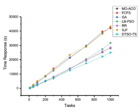
Response time: Figure 1 shows the response time for different task scheduling algorithms with various numbers of tasks. The response time is defined as the time it takes for a task to be completed from the moment it is submitted to the system. Minimizing response time is important for ensuring efficient task execution and good performance in cloud computing systems.
The DTSO-TS algorithm consistently had the lowest response time among the algorithms tested, with values ranging from 140.11 seconds for tasks of 10 to 5181.86 seconds for tasks of 200. Hence, this suggests that the DTSO-TS algorithm is able to carry out tasks in a shorter time than other algorithms. The highest response times were for tasks of 10, from the FCFS, GA [18] and SJF algorithms, being respectively 419.50 seconds for tasks of 10 to 8626.72 seconds for tasks of 200. This implies that these algorithims move rather slowly, perhaps because of how they order and assign tasks.
Figure 1. Response time comparison for different task scheduling algorithms
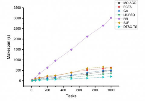
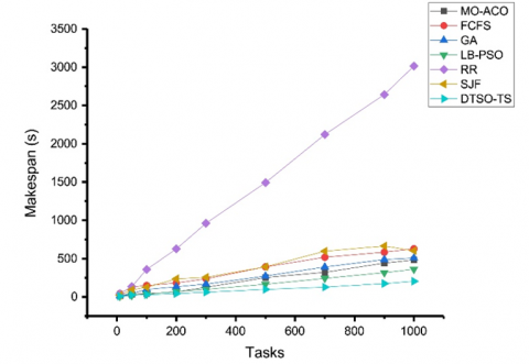
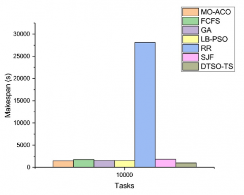
Makespan: Figure 2 depicts Makespan for different task scheduling algorithms with various task counts. Reducing Makespan is key for optimizing use of resources and performance in cloud computing systems. The DTSO-TS algorithm displayed the lowest Makespan values across tasks of 10, 50, 100, 200, and 300; with values ranging from 9 seconds for tasks of 10 up to 125 seconds for 300 tasks - evidence that it could complete tasks within shorter time frames than other algorithms. MO-ACO [16], GA [18], and LB-PSO [17] algorithms had relatively low Makespan values for tasks 10-50 but much higher Makespan values when applied to 100 or higher tasks. This suggests that these algorithms may be more efficient at handling smaller numbers of tasks but may become less so as their workload increases. FCFS, RR and SJF algorithms had the highest Makespan values ranging from 45 seconds for tasks of 10 up to 13778.99 seconds when dealing with 300 tasks. When dealing with 1000 tasks however, only the DTSO-TS algorithm achieved a lower Makespan of 204 seconds than all of the other algorithms - suggesting it can complete tasks relatively rapidly even when faced with high task volumes.
Throughput: Throughput can be defined as the number of tasks completed within a certain time period, and having high throughput is critical for optimizing resource utilization and increasing productivity within cloud computing systems. As illustrated by Figure 3, the DTSO-TS algorithm consistently had the highest throughput values for tasks 10, 50, and 100; its throughput values ranged from 0.75 to 4.14 tasks per second indicating its capability of handling multiple tasks quickly. MO-ACO [16] and LB-PSO [17] algorithms produced relatively high throughput values for tasks 10-50 but had lower throughput for 100+ tasks, whereas GA [18] and RR algorithms yielded low throughput values for all tasks, with values between 2.9-3.17 tasks per second. For 1000 tasks, the DTSO-TS algorithm had the highest throughput among all other algorithms at 5.99 tasks/second. This shows that it can complete more tasks more quickly compared to its counterparts.
Figure 2. Makespan comparison
Figure 3. Throughput
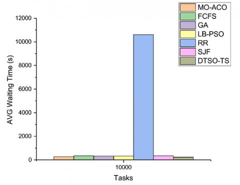
Average waiting time: The AWT measures how long tasks spend waiting to be assigned a resource. Figure 4 clearly displays the results of our tests of various algorithms; among those tested, the DTSO-TS algorithm consistently had the lowest average waiting time ranging from 0.38 seconds for tasks of 10 up to 74.79 seconds when testing 1000 tasks. This indicates that the DTSO-TS algorithm can allocate tasks and resources more rapidly compared to other algorithms, with MO-ACO [16] and LB-PSO [17] having generally shorter waiting times compared with FCFS, GA [18], and SJF. FCFS, GA [18], and SJF algorithms had the highest average waiting times; values ranged from 0.75 seconds for tasks of 10 up to 111.70 seconds when processing 1000 tasks. RR algorithms had particularly high average waiting times, ranging from 9.36 seconds for tasks of 10 up to 1383.11 seconds for 1000 tasks. This suggests that these algorithms may take longer to assign tasks to resources; decreasing this average waiting time is crucial to speeding up workload execution times and improving resource fairness.
Figure 4. AVG waiting time to resources
Our simulations show that the DTSO-TS algorithm consistently outperformed the other algorithms regarding response time makespan throughput and average waiting time this suggests that the DTSO-TS algorithm is more efficient at scheduling tasks in a cloud computing environment the lower response time and makespan values indicate that the DTSO-TS algorithm can complete tasks more quickly while the higher throughput values suggest that it can handle a larger number of tasks in a given time period.
6.2 Second scenario
In our second scenario, we increased the number of tasks from 1000 to 10000 and increased both hosts (9 total) and virtual machines (VMs), to 200 each in our simulation environment. This enabled us to further assess the efficiency of the DTSO-TS algorithm as well as assess its scalability in large-scale cloud computing environments.
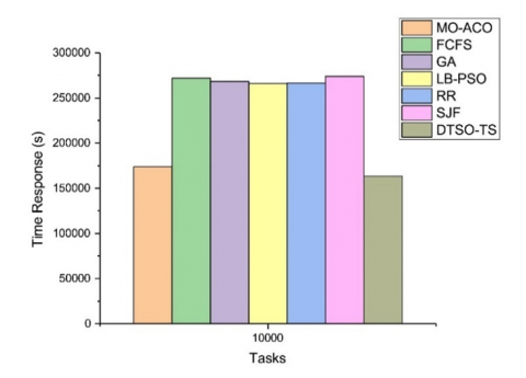
Figures 5-8 present the results of simulations showing how well the DTSO-TS algorithm performed for tasks of 10000 with regard to response time, Makespan and AVG waiting times as well as throughput value for all tested algorithms; its values being among the lowest of any algorithm tested; additionally, it had the highest throughput value among them all. Other algorithms like MO-ACO [16], GA [18], and LB-PSO [17] also achieved low values but lower throughput values compared with that of DTSO-TS while the FCFS, RR, and SJF algorithms had relatively high values for response time, Makespan, and AVG waiting time and lower throughput values compared to the DTSO-TS algorithm.
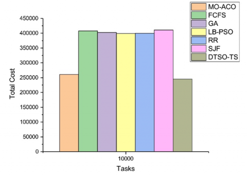
Total cost is a metric that measures the overall expense associated with performing all tasks within an environment, whether cloud computing or not. When used within cloud environments, total costs can vary based on factors like number of virtual machines deployed and amount of energy consumed to complete tasks. As demonstrated by Figure 9, our study revealed that DTSO-TS had the lowest total cost among all algorithms tested for task 10000 tasks; this indicated it to be relatively efficient with regards to resource utilization when compared to its counterparts. MO-ACO [16], GA [18], and LB-PSO [17] algorithms also had relatively low total cost values; FCFS, RR, and SJF algorithms exhibited higher costs; while overall the DTSO-TS algorithm displayed the least total costs among all algorithms tested; suggesting it as being most suitable to task scheduling in cloud environments.
Figure 10 provides a comparative analysis of the Makespan, a performance metric in task scheduling that represents the total completion time of all tasks, for the LB-PSO [17] and DTSO-TS algorithms over various numbers of iterations (from 10 to 100).
In the case of the LB-PSO [17] algorithm, a clear downward trend is visible in the Makespan as the number of iterations increases. The values decrease from 364.97118 at 10 iterations to 292.13193 at 100 iterations. This suggests an improvement in efficiency with more iterations, indicating that the algorithm requires less time to complete tasks. However, it is noteworthy that the global minima, the point at which the algorithm is most efficient, is not reached until after 60 iterations.
On the other hand, the DTSO-TS algorithm consistently shows lower Makespan values across all iteration counts, showing that it can complete tasks faster. Makespan for DTSO-TS decreases significantly from 174.78548 at 10 iterations to 143.56733 after 100 iterations; its global minima can be achieved as early as the 30th iteration, and Makespan does not change significantly thereafter, suggesting it reaches optimal efficiency earlier than LB-PSO [17] algorithm.
These observations demonstrate that the DTSO-TS algorithm outshone its counterpart, the LB-PSO [17], both in terms of Makespan values across all iteration counts tested, as well as reaching peak efficiency more quickly - evidence of its superior computational efficiency that makes it a sound choice regardless of iterations count.
Figure 5. Comparison of response time
Figure 6. Throughput
Figure 7. Makespan
Figure 8. AVG waiting time
From a performance point of view, DTSO-TS algorithm was superior to all the other algorithms; it had the lowest response time, Makespan, average waiting time, and highest throughput of any. This indicates that it excels at scheduling tasks as well as optimizing resource use in cloud computing environments. Other algorithms also performed competitively but could not match its efficiency especially as task numbers increased.
Figure 9. Comparison of the total cost for 10000 tasks using various algorithms
Figure 10. Depicts the convergence rate for both our proposed algorithm DTSO-TS and LB-PSO
An analysis of convergence rate showed that the DTSO-TS algorithm achieved its maximum efficiency faster than any of the other algorithms; this means it quickly finds optimal solutions - essential in cloud computing environments where tasks must be scheduled and completed on schedule.
This paper proposes an innovative task scheduling approach in cloud computing environments using a discrete version of Tuna Swarm Optimization for Task Scheduling (DTSO-TS) algorithm. Our approach stands out from others by adhering to its core principles; specifically optimizing task allocation to virtual machines while improving various performance metrics is at its heart.
Experimental validation demonstrates that the DTSO-TS algorithm significantly enhances workload balance and resource utilization, providing a competitive edge in cloud computing environments for task scheduling. With high throughput and resource utilization achieved by this algorithm, its high throughput directly impacts efficiency and performance metrics directly influencing cloud environments - leading to cost savings and enhanced service delivery.
Note, however, that our current work makes certain assumptions which could alter its conclusions. For instance, we assume a stable cloud environment with no network failures or resource outages; real world implementations need to account for such factors. Looking ahead, we see an opportunity for further investigation of how changing random variable parameters impact DTSO-TS's performance.
We also suggest exploring new problem formulations, techniques, and extensions to the DTSO-TS algorithm. A comparative study between the DTSO-TS and other bio-inspired optimization algorithms for task scheduling could yield valuable insights, further driving the evolution of cloud computing environments.
In conclusion, the DTSO-TS algorithm offers promising opportunities for implementation and further scrutiny within real-world contexts, reinforcing its applicability and potential impact on the field.
|
TSO |
Tuna Swarm Optimization |
|
DTSO-TS |
Discrete Tuna Swarm Optimization for Task Scheduling) - A modified version of the TSO algorithm that works with discrete values, suitable for task scheduling problems. |
|
t |
Current iteration |
|
Xbest |
The best position (solution) found so far during the optimization process. |
|
Xrand |
A randomly selected position from the population. |
|
$X_i^t$ |
The position of the i-th tuna at time t |
|
tmax |
The maximum number of iterations allowed in the algorithm. |
|
NP |
The number of particles in the population. |
|
w1 |
Weight assigned to Makespan in the fitness function. |
|
w2 |
Weight assigned to average utilization in the fitness function. |
|
w3 |
Weight assigned to total completion time (Total CT) in the fitness function. |
|
TF |
A parameter used in Eq. (18) to adjust the influence of the global best position on the update of a particle’s position. |
|
$\circledast, \ominus, \oplus$ |
New operators introduced in the DTSO-TS algorithm to handle discrete values and maintain the stochastic nature of the algorithm. |
|
p |
A random value between 0 and 1. |
|
Greek symbols |
|
|
α1, α2 |
Tunable parameters that control the balance between exploration and exploitation in the algorithm. |
|
β |
A scaling factor applied to the difference between the best position and the current position. |
[1] Armbrust, M., Fox, A., Griffith, R., Joseph, A.D., Katz, R., Konwinski, A., Lee, G., Patterson, D., Rabkin, A., Stoica, I., Zaharia, M. (2010). A view of cloud computing. Communications of the ACM, 53(4): 50-58. https://doi.org/10.1145/1721654.1721672
[2] Abid, A., Manzoor, M.F., Farooq, M.S., Farooq, U., Hussain, M. (2020). Challenges and issues of resource allocation techniques in cloud computing. KSII Transactions on Internet & Information Systems, 14(7): 2815–39. https://doi.org/10.3837/tiis.2020.07.005
[3] Goudarzi, H., Pedram, M. (2011). Maximizing profit in cloud computing system via resource allocation. In 2011 31st International Conference on Distributed Computing Systems Workshops, Minneapolis, MN, USA, pp. 1-6. https://doi.org/10.1109/ICDCSW.2011.52
[4] Masdari, M., Salehi, F., Jalali, M., Bidaki, M. (2017). A survey of PSO-based scheduling algorithms in cloud computing. Journal of Network and Systems Management, 25(1): 122-158. https://doi.org/10.1007/s10922-016-9385-9
[5] Kantale, V. (2020). Statistical evaluation of task scheduling algorithms in cloud environments. IJATCSE, 9: 1486–90. https://doi.org/10.30534/ijatcse/2020/88922020
[6] Maniyar, B., Kanani, B. (2015). Review on round robin algorithm for task scheduling in cloud computing. Journal of Emerging Technologies and Innovative Research, 2(3): 788-893.
[7] Xie, L., Han, T., Zhou, H., Zhang, Z.R., Han, B., Tang, A. (2021). Tuna swarm optimization: A novel swarm-based metaheuristic algorithm for global optimization. Computational intelligence and Neuroscience, 2021: 1-22. https://doi.org/10.1155/2021/9210050
[8] Raj, B., Ranjan, P., Rizvi, N., Pranav, P., Paul, S. (2018). Improvised bat algorithm for load balancing-based task scheduling. In Progress in Intelligent Computing Techniques: Theory, Practice, and Applications: Proceedings of ICACNI 2016, pp. 521-530. https://doi.org/10.1007/978-981-10-3373-5_52
[9] Alzaqebah, A., Al-Sayyed, R., Masadeh, R. (2019). Task scheduling based on modified grey wolf optimizer in cloud computing environment. In 2019 2nd International Conference on new Trends in Computing Sciences (ICTCS), Amman, Jordan, pp. 1-6. https://doi.org/10.1109/ICTCS.2019.8923071
[10] Asghari, S., Jafari Navimipour, N. (2023). The role of an ant colony optimisation algorithm in solving the major issues of the cloud computing. Journal of Experimental & Theoretical Artificial Intelligence, 35(6): 755-790. https://doi.org/10.1080/0952813X.2021.1966841
[11] Neelima, P., Reddy, A.R.M. (2020). An efficient load balancing system using adaptive dragonfly algorithm in cloud computing. Cluster Computing, 23: 2891-2899. https://doi.org/10.1007/s10586-020-03054-w
[12] Mahmood, A., Khan, S.A., Bahlool, R.A. (2017). Hard real-time task scheduling in cloud computing using an adaptive genetic algorithm. Computers, 6(2): 15. https://doi.org/10.3390/computers6020015
[13] Ullah, A., Nawi, N.M., Uddin, J., Baseer, S., Rashed, A.H. (2019). Artificial bee colony algorithm used for load balancing in cloud computing: Review. IAES International Journal of Artificial Intelligence, 8: 156–167. https://doi.org/10.11591/ijai.v8.i2.pp%p
[14] Awad, A.I., El-Hefnawy, N.A., Abdel_kader, H.M. (2015). Enhanced particle swarm optimization for task scheduling in cloud computing environments. Procedia Computer Science, 65: 920-929. https://doi.org/10.1016/j.procs.2015.09.064
[15] Calheiros, R.N., Ranjan, R., Beloglazov, A., De Rose, C.A., Buyya, R. (2011). CloudSim: A toolkit for modeling and simulation of cloud computing environments and evaluation of resource provisioning algorithms. Software: Practice and Experience, 41(1): 23-50. https://doi.org/10.1002/spe.995
[16] Guo, Q. (2017). Task scheduling based on ant colony optimization in cloud environment. In AIP Conference Proceedings, 1834(1): 040039. https://doi.org/10.1063/1.4981635
[17] Ebadifard, F., Babamir, S.M. (2018). A PSO-based task scheduling algorithm improved using a load-balancing technique for the cloud computing environment. Concurrency and Computation: Practice and Experience, 30(12): e4368. https://doi.org/10.1002/cpe.4368
[18] Dasgupta, K., Mandal, B., Dutta, P., Mandal, J.K., Dam, S. (2013). A genetic algorithm (GA) based load balancing strategy for cloud computing. Procedia Technology, 10: 340-347. https://doi.org/10.1016/j.protcy.2013.12.369
[19] Ghomi, E.J., Rahmani, A.M., Qader, N.N. (2017). Load-balancing algorithms in cloud computing: A survey. Journal of Network and Computer Applications, 88: 50-71. https://doi.org/10.1016/j.jnca.2017.04.007
[20] Fang, Y., Wang, F., Ge, J. (2010). A task scheduling algorithm based on load balancing in cloud computing. In Web Information Systems and Mining: International Conference, WISM 2010, Sanya, China, October 23-24, 2010. Proceedings, pp. 271-277. https://doi.org/10.1007/978-3-642-16515-3_34
[21] Lakra, A.V., Yadav, D.K. (2015). Multi-objective tasks scheduling algorithm for cloud computing throughput optimization. Procedia Computer Science, 48: 107-113. https://doi.org/10.1016/j.procs.2015.04.158
[22] Pal, S., Pattnaik, P.K. (2016). Adaptation of Johnson sequencing algorithm for job scheduling to minimise the average waiting time in cloud computing environment. Journal of Engineering Science and Technology, 11(9): 1282-1295.
[23] Sefati, S., Mousavinasab, M., Zareh Farkhady, R. (2022). Load balancing in cloud computing environment using the Grey wolf optimization algorithm based on the reliability: Performance evaluation. The Journal of Supercomputing, 78(1): 18-42. https://doi.org/10.1007/s11227-021-03810-8
[24] Mishra, K., Majhi, S.K. (2021). A binary Bird Swarm Optimization based load balancing algorithm for cloud computing environment. Open Computer Science, 11(1): 146-160. https://doi.org/10.1515/comp-2020-0215
[25] Ebadifard, F., Babamir, S.M., Barani, S. (2020). A dynamic task scheduling algorithm improved by load balancing in cloud computing. In 2020 6th International Conference on Web Research (ICWR), pp. 177-183. https://doi.org/10.1109/icwr49608.2020.9122287
[26] Devaraj, A.F.S., Elhoseny, M., Dhanasekaran, S., Lydia, E.L., Shankar, K. (2020). Hybridization of firefly and improved multi-objective particle swarm optimization algorithm for energy efficient load balancing in cloud computing environments. Journal of Parallel and Distributed Computing, 142: 36-45. https://doi.org/10.1016/j.jpdc.2020.03.022
[27] Latchoumi, T.P., Parthiban, L. (2022). Quasi oppositional dragonfly algorithm for load balancing in cloud computing environment. Wireless Personal Communications, 122(3): 2639-2656. https://doi.org/10.1007/s11277-021-09022-w
[28] Singh, H., Tyagi, S., Kumar, P. (2021). Cloud resource mapping through crow search inspired metaheuristic load balancing technique. Computers & Electrical Engineering, 93: 107221. https://doi.org/10.1016/j.compeleceng.2021.107221
[29] Mangalampalli, S., Swain, S.K., Mangalampalli, V.K. (2022). Prioritized energy efficient task scheduling algorithm in cloud computing using whale optimization algorithm. Wireless Personal Communications, 126(3): 2231-2247. https://doi.org/10.1007/s11277-021-09018-6
[30] Yakhchi, M., Ghafari, S.M., Yakhchi, S., Fazeli, M., Patooghi, A. (2015). Proposing a load balancing method based on Cuckoo Optimization Algorithm for energy management in cloud computing infrastructures. In 2015 6th International Conference on Modeling, Simulation, and Applied Optimization (ICMSAO), pp. 1-5. https://doi.org/10.1109/ICMSAO.2015.7152209
[31] Calheiros, R.N., Ranjan, R., De Rose, C.A., Buyya, R. (2009). Cloudsim: A novel framework for modeling and simulation of cloud computing infrastructures and services. arXiv preprint arXiv:0903.2525. https://doi.org/10.48550/arXiv.0903.2525